Life Insurance Capital Adequacy Test (2023) - Chapter 7 Segregated Fund Guarantee Risk

Information

Publication type

Guideline

7.1. Products

Guaranteed Minimum Death Benefit (GMDB) forms modeled include the following:

Return of Premium (ROP): provides a death benefit guarantee equal to the higher of the account value or the premiums paid.
5% Annual Roll-up (ROLL): provides a guaranteed benefit that increases 5% per annum compounded at each contract anniversary with the guarantee frozen at age 80.
Maximum Anniversary Value/Annual Ratchet (MAV): automatic annual reset of guarantee at each contract anniversary with resets frozen at age 80.
10-year Rollover Contract (GMDB_10): guarantee can reset and term-to-maturity also will reset to 10 years. No resets are permitted in the final 10 years prior to contract maturity.

Guaranteed Minimum Maturity Benefits (GMMB) forms modeled include:

Fixed Maturity Date (FIXED): guarantee is level and applies up to the fixed maturity date.
10-year Rollover Maturity Benefit (GMMB_10): guarantee can be reset and term-to-maturity also resets to 10 years. No resets are permitted in the 10 years prior to contract maturity.
Guaranteed Minimum Surrender Benefit After 10 Years (GMSB_10): guarantee comes into effect 10 years after contract issue. If the guaranteed value at 10 years is greater than the account value at surrender, a "top-up" benefit equal to the difference is paid.

7.2. Documentation and reporting

The columns of the reporting form on page 70.100 are completed as follows:

Column 01 - Guaranteed Value

This is the amount guaranteed in all segregated funds. If the funds are subject to guarantees of differing amounts, for example 100% on death and 75% on maturity, report the larger amount here.

Column 02 - Market Value

This is the market value of all segregated funds.

Column 03 - Total Gross Calculated Requirements

This is the total gross calculated requirement for all segregated funds.

Column 04 - Credit for Reinsurance Ceded

Report credit for amounts ceded in column 04. Note that aggregate positive liabilities ceded under unregistered reinsurance (q.v. section 10.1), net of the available credit for reinsurance (q.v. section 10.3), must be deducted from Available Capital/Margin on page 20.030 of the LICAT Quarterly Return or LICAT Annual Supplement. Eligible Deposits held for unregistered reinsurance, for a period not less than the remaining guarantee term, may be recognized subject to the limit in section 6.8.1.

Column 05 - Net Requirements

This is determined as:

(Total Gross Calculated Requirements − Credit for Reinsurance Ceded)

Column 06 – Credit for OSFI-Approved Hedging Programs

This is the dollar equivalent of the maximum allowable reduction. It is determined as:

(Maximum allowable percentage reduction × Net Requirements)

where the maximum percentage reduction is the reduction that was determined at the time of approval. See the OSFI Advisory: Recognition of Hedge Contracts in the Determination of the Segregated Fund Guarantee Capital Requirement for Life Insurance Companies dated December 2008.

This column may also be used to enter the amount of a negative Guaranteed Minimum Withdrawal Benefit Hedging Liability (enter the amount as a positive value in this column) to effectively floor this negative value at zero in determining the Net Required Component in Column 8.

Column 07 - Net Actuarial Liabilities Held

This is the total net actuarial liability (including risk adjustment and contractual service margin) held on the balance sheet for segregated fund contracts with guarantee risks.

Column 08 - Net Required Component

This is determined as:

(Net Requirements (column 5) − Credit for OSFI-Approved Hedging Programs (column 6) − Net Actuarial Liabilities Held (column 7)) × 1.25

The net required component is multiplied by 1.25 to bring required capital to the supervisory target level.

Line 920 must not be less than zero in total.

The columns of the reporting form on page 70.200 are completed as follows:

Column 01 - Factor Requirements on Business

This is the gross calculated requirement based on the OSFI-approved factors.

Column 02 - OSFI Approved Internal Model Requirements

For OSFI-approved models, this is the gross calculated requirement based on company-specific internal models.

Column 03 - Total Gross Calculated Requirements

For OSFI-approved models, transition rules apply:

In the first year of approval, Total Gross Calculated Requirements = 50% of the Factor Requirements + 50% of the Internal Model Requirements.

Thereafter, Total Gross Calculated Requirements = 100% of the Internal Model Requirements.

Otherwise, Total Gross Calculated Requirements = 100% of the Factor Requirements.

Column 04 - Credit for Reinsurance Ceded

Column 05 - Net Requirements

This is determined as:

(Total Gross Calculated Requirements (column 3) − Credit for Reinsurance Ceded (column 4))

Column 06 - Credit for OSFI-Approved Hedging Programs

This is the dollar equivalent of the maximum allowable reduction. It is determined as:

(Maximum allowable percentage reduction × Net Requirements (column 5))

Column 07 - Net Actuarial Liabilities Held

This is the total net actuarial liability (including risk adjustment and contractual service margin) held on the balance sheet for segregated fund contracts with guarantee risks.

Column 08 - Net Required Component

This is determined as:

(Net Requirements (column 5) − Credit for OSFI Approved Hedging Programs (column 6) − Net Actuarial Liabilities Held (column 7)) × 1.25

The net required component is multiplied by 1.25 to bring required capital to the supervisory target level.

Note that the amount reported on page 70.100, column 08 should be the same as the amount reported on page 70.200, column 08.

7.3. Total gross calculated requirement

7.3.1. Overview

It is expected that the LICAT methodology for Total Gross Calculated Requirement (" TGCR ") will be applied on a policy-by-policy basis (i.e., seriatim). If the company adopts a cell-based approach, only materially similar contracts should be grouped together. Specifically, all policies composing a "cell" must display substantially similar characteristics for those attributes expected to affect risk-based capital (e.g., definition of guaranteed benefits, attained age, policy duration, years-to-maturity, market-to-guaranteed value, and asset mix). The TGCR for the purpose of determining capital requirements for segregated funds using prescribed or approved factors should not include deferred income taxes.

The portfolio TGCR is the sum of the TGCR calculations for each policy or cell. The result for any given policy (cell) may be negative, zero or positive. In total, the TGCR cannot be negative.

The TGCR for a given policy is equal to:

$TGCR = GV \times \hat{f} (\tilde{θ}) - AV \times \hat{g} (\tilde{θ})$

where:

GV = current guaranteed minimum benefit,
AV = current account balance,
$\hat{f} (\tilde{θ})$ = benefit cost factor,
$\hat{g} (\tilde{θ})$ = margin offset factor and
$\tilde{θ}$ is a vector that defines the risk characteristics for the policy.

The factors $\hat{f} (\tilde{θ})$ and $\hat{g} (\tilde{θ})$ are described more fully in section 7.7.1. The TGCR is calculated separately for each guaranteed minimum benefit (i.e., death, maturity and surrender).

The model assumptions for the TGCR Factors are documented in section 7.3.2.

There are four (4) major steps in determining the TGCR for a given policy/cell:

Classify the asset exposure (section 7.4);
Determine the risk attributes (section 7.5);
Retrieve the appropriate nodes (section 7.6);
Use the supplied functions to determine the requirement (section 7.7).

The first step requires the company to categorize the asset value for the given policy/cell by mapping the entire exposure to one of the prescribed "fund classes" as described in section 7.4. TGCR factors are provided for each asset class.

The second step requires the company to determine (or derive) the appropriate attributes for the given policy or cell. The attributes needed to access the factor tables and calculate the required values are:

Product form ("Guarantee Definition"), P .
Guarantee level, G .
Adjustment to guaranteed value upon partial withdrawal ("GMDB/GMMB Adjustment"), A .
Fund class, F .
Attained age of the policyholder, X , (for GMDB only, use a 4-year setback for female lives).
Contract maturity age, M , (for GMDB only, use a 4-year setback for female lives).
Time-to-next maturity date, T .
Ratio of account value to guaranteed value, Ø .
Total "equivalent" account-based charges, MER ("management expense ratio").
Reset utilization rate, R (where applicable).
In-the-money termination rate, S (guaranteed surrender benefits only).

Other required policy values include:

Total account value on which the guaranteed benefit is calculated, AV .
Current GMDB , GMMB and/or GMSB .
Total net spread available to fund guaranteed benefits ("margin offset"), α .

The next steps – retrieving the appropriate nodes and using the supplied functions to determine the requirement – are explained in sections 7.6 and 7.7. Software tools have been developed to assist companies in these efforts. If an insurer is unable to use the supplied tools, it will be required to develop software of its own. In such a situation, the insurer should contact OSFI for specific guidance on how to develop its own lookup and extraction routines. A calculation example demonstrating the application of the various component factors to a sample policy is provided in section 7.7.2.

In this chapter, GMDB , GMMB , GMSB are generically denoted by GV . AV generically denotes either Account Value or Market Value. The total "equivalent" account charges should include all amounts assessed against policyholder accounts, expressed as a level spread per year (in basis points). This quantity is called the Management Expense Ratio ("MER") and is defined as the average amount (in dollars) charged against policyholder funds in a given year divided by average account value. Normally, the MER would vary by fund class and be the sum of investment management fees, mortality & expense charges, guarantee fees/risk premiums, and other items. The total spread available to fund the guaranteed benefits (i.e., GMDB, GMMB, GMSB costs) is called the "margin offset" (denoted by α) and should be net of spread-based costs and expenses (e.g., net of maintenance expenses, investment management fees, trailer commissions, and amounts required to provide for amortization of deferred acquisition costs). Section 7.8 describes how to determine MER and α.

The GMDB/GMMB/GMSB definition for a given policy/cell may not exactly correspond to those provided. In some cases, it may be reasonable to use the factors/formulas for a different product form. In other cases, the company might determine the TGCR based on two different guarantee definitions and interpolate the results to obtain an appropriate value for the given policy/cell. However, if the policy form is sufficiently different from those provided and there is no practical or obvious way to obtain a reasonable result, the insurer should follow the instructions outlined in section 7.10.

The general form of the TGCR may be written as:

$TGCR = GV \times h (\tilde{θ}) \times w (\tilde{θ}) \times f (\tilde{θ}) - \frac{α}{100} \times AV \times g (\tilde{θ})$

where:

GV = current guaranteed minimum benefit (dollars)
AV = current account value (dollars)
$f (\tilde{θ})$ = cost factor per $1 of GV
$g (\tilde{θ})$ = margin offset factor per $1 of AV (assuming 100 bps of available spread)
$h (\tilde{θ})$ = asset mix diversification factor
$w (\tilde{θ})$ = time diversification factor

Under this notation, $\tilde{θ}$ is used to generically represent the risk attribute set (e.g., product form, guaranteed level, asset class, attained age, etc.) for the policy, or some relevant subset thereof. α is the company-determined net spread ("margin offset", in basis points per annum) available to fund the guaranteed benefits.

Where more than one feature (i.e., guaranteed benefit) is present in a product, unless the company has a justifiable alternative for allocating the total available spread between the benefit types (e.g. explicitly defined risk charges), the split should be based on the proportionate gross guaranteed benefit costs. An example is provided in section 7.7.2 to illustrate this concept.

In practice, $f (\tilde{θ})$ , $g (\tilde{θ})$ , $h (\tilde{θ})$ and $w (\tilde{θ})$ are values interpolated from the factor grid. The use of the factor grid is discussed more fully in section 7.7. The factor grid is a large pre-computed table developed using stochastic modeling for a wide array of combinations of the risk attribute set. The risk attribute set is defined by those policy/product characteristics that affect the risk profile (exposure) of the business: product form (guarantee definition), fund class, attained age, AV/GV ratio, time-to-maturity, etc.

7.3.2. Assumptions for TGCR methodology published factors

Each node in the factor grid is effectively the modeled result for a given "cell" assuming a $100 single deposit.

Table 1: Model Assumptions & Product Characteristics
Account Charges (MER)	Vary by fund class. See Table 2 later in this section.
Base Margin Offset	100 basis points per annum.
GMDB Description	ROP = return of premium. ROLL = 5% compound roll-up, frozen at age 80. MAV = annual ratchet (maximum anniversary value), frozen at age 80. GMDB_10 = 10-year rollover contract.
GMMB & GMSB Descriptions	FIXED = fixed maturity date. GMSB_10 = 10-year guaranteed surrender benefit. GMMB_10 = 10-year rollover maturity benefit.
GV Adjustment on Withdrawal	"Pro-Rata by Market Value" and "Dollar-for-Dollar" are tested separately.
Surrender Charges	Ignored (i.e., zero).
Base Policy Lapse Rate	6% p.a. at all policy durations. See also "Dynamic Lapse Multiplier".
Partial Withdrawals	Flat 4% p.a. at all policy durations (as a % of AV). No dynamics.
Rollover (Renewal) Rate	85% at the end of each 10-year term (GMDB_10 and GMMB_10 only).
Dynamic Lapse Multiplier	Actual lapse rate = λ× [ Base Policy Lapse Rate ], where: $λ = MIN [λ^{+}, MAX [λ^{-}, [a + b \times (\frac{AV}{GV})] \times [c + d \times MIN (h, T)]]]$ λ⁺ = 1.6667, λ^- = 0.3333, `a` = -0.0952, `b` = 0.8010, `c` = 0.6279, `d` = 0.0654 `h` = 10 and `T` = time-to-next maturity
Mortality	100% of CIA 1986–92 ALB Male Aggregate Ultimate.
Fixed Expenses, Annual Fees	Ignored (i.e. zero).
Discount Rate	5.5% annual effective (non-dynamic).
Elective Reset of GV	Whenever the AV/GV ratio exceeds 115% (maximum 2 resets per year). No resets are permitted in the 10 years prior to the final "contract" maturity date.
In-The-Money Surrender (GMSB_10 only)	Whenever the benefit is payable (i.e., 10 years after issue or last reset) and the AV/GV ratio is less 85%.

Notes on Factor Development:

The GMDB roll-up is compounded (not simple interest, not stepped at each anniversary) and is applied to the previous roll-up guaranteed value.
The "Base Policy Lapse Rate" is the rate of policy termination (surrenders). Policy terminations (surrenders) are assumed to occur throughout the policy year (not only on anniversaries).
Partial withdrawals are assumed to occur at the end of each time period (quarterly).
Account charges ("MER") represent the total amount (annualized, in basis points) assessed against policyholder funds (e.g., sum of investment management fees, mortality and expense charges, risk premiums, and policy/administrative fees). They are assumed to occur throughout the policy year (not only on anniversaries).
For the GMDB_10 and GMMB_10 products, the contract rolls over (renews) at the end of each 10-year term for another 10 years. The guaranteed benefit resets to Z% of MV (after payment of any top-up maturity benefit for in-the-money maturity guarantees) where Z is typically 75 or 100.
The guaranteed minimum surrender benefit (GMSB_10) comes into effect 10 years after contract issue. If the guaranteed value at 10 years is greater than the account value at surrender, a "top-up" benefit equal to the difference is paid.

Table 2: Account-Based Fund Charges (bps per annum)
Asset Class / Fund	Account Value Charges (MER)
Money Market	110
Fixed Income (Bond)	200
Balanced	250
Low Volatility Equity	265
Diversified Equity	265
Intermediate Risk Equity	280
Aggressive or Exotic Equity	295

The annualized total fund depletion rates (i.e., including the fixed 4% per annum partial withdrawal) are illustrated in Figure 1 for various AV/GV ratios and times to maturity.

Figure 1: Fund Depletion Rates (Lapse + Partial Withdrawal) by AV/GV Ratio & Time-to-Maturity

Total Annualized Fund Depletion Rate. Chart description below.

Total Annualized Fund Depletion Rate - Chart description

The graph shows annualized fund depletion rates (lapses plus partial withdrawals) by time to maturity for six different levels of AV/GV. When AV/GV is 0.5, the depletion rate is approximately 6% for all times to maturity. When AV/GV is 1, the depletion rate starts at 6.5% for maturity zero and increases linearly to 9.5% at maturities 10 years and higher. When AV/GV is 1.75, the depletion rate starts at 9% for maturity zero and increases linearly to 14% at maturities 10 years and higher.

7.4. Classifying the asset exposure

7.4.1. Definition of asset classes

Where data for the fund or benchmark are too sparse or unreliable, the fund exposure should be moved to the next higher volatility class than otherwise indicated. In reviewing the asset classifications, care should be taken to reflect any additional volatility of returns added by the presence of currency risk, liquidity (bid-ask) effects, short selling and speculative positions.

All exposures/funds must be categorized into one of the following seven (7) asset classes:

Money Market/Short-Term
Fixed Income
Balanced
Low Volatility Equity
Broad-Based Diversified Equity
Intermediate Risk Equity
Aggressive or Exotic Equity

Money Market/Short-Term

The fund is invested in money market instruments with an average remaining term-to-maturity of less than 365 days.

Fixed Income

The fund is invested primarily in investment grade fixed income securities. Up to 25% of the fund within this class may be invested in diversified equities or high-yield bonds. The expected volatility of the fund returns will be lower than the Balanced fund class.

Balanced

This class is a combination of fixed income securities with a larger equity component. The fixed income component should exceed 25% of the portfolio. Additionally, any aggressive or 'specialized' equity component should not exceed one-third (33.3%) of the total equities held. Should the fund violate either of these constraints, it should be categorized as an equity fund. These funds usually have a long-term volatility in the range of 8% − 13%.

Low Volatility Equity

The expected volatility of the fund should be less than 15.5% (annualized) and the aggressive/exotic equity component of the equity holdings should be less than 33.3% of the total equities by market value. Further, the overall asset holdings should satisfy at least one of the following conditions:

The fund permanently maintains a relatively large cash or fixed income position (greater than 10% of the market value of assets) as part of its investment strategy;
The fund is "income" oriented and contains a significant (greater than 10% of the market value of assets) proportion of stocks paying material and regular dividends that are automatically reinvested in the fund.

Broad-Based Diversified Equity

The fund is invested in a well-diversified mix of Canadian, U.S. or global equities. The foreign equity component must be comprised of liquid securities in well-developed markets. Funds in this category would exhibit long-term volatility comparable to that of the TSX. These funds should usually have a long-term volatility in the range of 13% − 19%.

Intermediate Risk Equity

The fund has a mix of characteristics from both the Diversified and Aggressive Equity Classes. These funds have a long-term volatility in the range of 19% − 25%.

Aggressive or Exotic Equity

This class comprises more volatile funds where risk can arise from: (a) underdeveloped markets, (b) uncertain markets, (c) high volatility of returns, (d) narrow focus (e.g., specific market sector), and other sources. The fund (or market benchmark) either does not have sufficient history to allow for the calculation of a long-term expected volatility, or the volatility is very high. This class would be used whenever the long-term expected annualized volatility is indeterminable or exceeds 25%.

7.4.2. Selecting appropriate investment classes

A seriatim process is used to identify the "grouped" fund holdings, to assess the risk profile of the current fund holdings (possibly calculating the expected long-term volatility of the funds held with reference to the indicated market proxies), and to classify the entire "asset exposure" into one of the specified choices. Here, "asset exposure" refers to the underlying assets (segregated and/or general account investment options) on which the guarantee will be determined. For example, if the guarantee applies separately for each deposit year within the contract, then the classification process would be applied separately for the exposure of each deposit year.

In summary, mapping the benefit exposure (i.e., the asset exposure that applies to the calculation of the guaranteed minimum benefits) to one of the prescribed asset classes is a multi-step process:

Map each separate and/or general account investment option to one of the prescribed asset classes. For some funds, this mapping will be obvious, but for others it will involve a review of the fund's investment policy, performance benchmarks, composition and expected long-term volatility.
Combine the mapped exposure to determine the expected long-term volatility of current fund holdings. This will require a calculation based on the expected long-term volatilities for each fund and the correlations between the prescribed asset classes as given in Table 3.
Evaluate the asset composition and expected volatility (as calculated in step 2) of current holdings to determine the single asset class that best represents the exposure, with due consideration to the constraints and guidelines presented earlier in this section.

In step 1, the company should use the fund’s actual experience (i.e., historical performance, inclusive of reinvestment) only as a guide in determining the expected long-term volatility. Due to limited data and changes in investment objectives, style and/or management (e.g., fund mergers, revised investment policy, and different fund managers), the company may need to give more weight to the expected long-term volatility of the fund’s benchmarks. In general, the company should exercise caution and not be overly optimistic in assuming that future returns will consistently be less volatile than the underlying markets.

In step 2, the company should calculate the "volatility of current fund holdings" ( for the exposure being categorized) by the following formula using the volatilities and correlations in Table 3.

$σ = \sqrt{Σ_{i = 1}^{n} Σ_{j = 1}^{n} w_{i} w_{j} ρ_{i j} σ_{i} σ_{j}}$

where $w_{i} = \frac{{AV}_{i}}{\underset{k}{Σ} {AV}_{k}}$ is the relative value of fund i expressed as a proportion of total contract value, ρ_ij is the correlation between asset classes i and j and σ_i is the volatility of asset class i (see Table 3).

Table 3: Volatilities and Correlations for Prescribed Asset Classes
Annual Volatility	blank	General Account	Money Market	Fixed Income	Balanced	Low Vol Equity	Diverse Equity	Interm Equity	AGGR Equity
1%	General Account	1	0.50	0.15	0	0	0	0	0
1%	Money Market	0.50	1	0.20	0	0	0	0	0
6%	Fixed Income	0.15	0.20	1	0.50	0.25	0.25	0.20	0.10
11%	Balanced	0	0	0.50	1	0.80	0.95	0.75	0.65
15%	Low Vol Equity	0	0	0.25	0.80	1	0.80	0.75	0.65
17%	Diverse Equity	0	0	0.25	0.95	0.80	1	0.75	0.65
22%	Interm Equity	0	0	0.20	0.75	0.75	0.75	1	0.70
26%	AGGR Equity	0	0	0.10	0.65	0.65	0.65	0.70	1

Example: Fund Categorization

blank	1	2	3	4	5
MV Fund X (Fixed Income):	5,000	6,000	8,000	-blank	5,000
MV Fund Y (Diversified Equity):	9,000	5,000	2,000	5,000	-blank
MV Fund Z (Aggressive Equity):	1,000	4,000	-blank	5,000	5,000
Total Market Value:	$15,000	$15,000	$10,000	$10,000	$10,000
Total Equity Market Value:	$10,000	$9,000	$2,000	$10,000	$5,000
Fixed Income % ( `A` ):	33%	40%	80%	0%	50%
Fixed Income Test ( `A` >75%):	No	No	Yes	No	No
Aggressive % of Equity (B):	10%	44%	n/a	50%	100%
Balanced Test ( `A` >25% & `B` <33.3%):	Yes	No	n/a	No	No
Volatility of Current Fund Holdings:	12.0%	12.1%	6.5%	19.6%	13.6%
Fund Classification:	Balanced	Diversified^{Footnote 1}	Fixed Income	Intermediate	Diversified

The "Volatility of Fund Holdings" for policy #1 is calculated as $\sqrt{A + B} = 12.04%$ where:

$\begin{array}{l} A & = {(\frac{5}{15} \times 0.06)}^{2} + {(\frac{9}{15} \times 0.17)}^{2} + {(\frac{1}{15} \times 0.26)}^{2} \\ = 1.1104% \\ B & = 2 \cdot (\frac{5}{15} \cdot \frac{9}{15}) (0.25 \times 0.06 \times 0.17) + 2 \cdot (\frac{5}{15} \cdot \frac{1}{15}) (0.10 \times 0.06 \times 0.26) + 2 \cdot (\frac{9}{15} \cdot \frac{1}{15}) (0.65 \times 0.17 \times 0.26) \\ = 0.3388% \end{array}$

Importantly, the volatility would be understated if we assumed zero correlation (e.g. if all market returns are independent) since B contributes materially to the final value.

7.5. Determining the risk attributes

The "Tabular" approach for the TGCR component creates a multi-dimensional grid (array) by testing a very large number of combinations for the policy attributes. The results are expressed as factors. The TGCR is calculated by looking into (based on a "key") the large, pre-computed multi-dimensional tables and using multi-dimensional linear interpolation. The lookup "key" depends on the risk attributes for the policy $\tilde{θ}$ = ( P , G , A , F , X , M , T , Φ , Δ , R , S ) where Φ is the AV/GV ratio for the benefit exposure under consideration, Δ is the "MER Delta", R is the utilization rate of the elective reset option (if applicable) and S is the "in-the-money" termination rate on GMSB_10 policies. The "MER Delta" is calculated based on the difference between the actual MER and that assumed in the factor testing (see Table 2), subject to a cap (floor) of 100 bps (-100 bps). See Table 4 for more details.

For GMDB, there are 4 × 2 × 2 × 7 × 4 × 4 × 5 × 7 × 3 × 2 = 376,320 "nodes" in the "Basic Factor" grid. Interpolation will only be permitted across the six (6) dimensions: Contract Maturity Age ( M ), Attained Age ( X ), Time to Next Maturity ( T ), AV/GV Ratio (Φ), MER Delta (Δ) and Reset Utilization Rate ( R ). The "In-the-Money" termination rate ( S ) is not used for GMDBs.

For GMMB, there are 3 × 2 × 2 × 7 × 1 × 7 × 5 × 7 × 3 × 2 × 2 = 246,960 "nodes" in the "Basic Factor" grid. Interpolation will only be permitted across the six (6) dimensions: Contract Maturity Age ( M ), Time to Next Maturity ( T ), AV/GV Ratio (Φ), MER Delta (Δ), Reset Utilization Rate ( R ) and In-the-Money Termination Rate ( S ). The "In-the-Money" termination rate ( S ) is only applies to the "GMSB_10" product form. The testing for guaranteed minimum maturity and surrender benefits assumed all lives were attained age 55 at the calculation date.

Functions are available to assist the company in applying the TGCR Methodology. More fully described in section 7.7, these functions perform the necessary factor table lookups and associated multi-dimensional linear interpolations. If the insurer is unable to use the supplied functions, it will be required to develop its own. In such a case, the insurer should contact OSFI for specific details.

The GMDB and GMMB/GMSB factors are respectively contained in the files "GMDBFactors_CTE95.csv" and "GMMBFactors_CTE95.csv". These are comma-separated value text files where each "row" represents the factors for a test policy as identified by its lookup key. Rows are terminated by new line and line feed characters. Factors are also provided at the CTE80 confidence level – the factor files are "GMDBFactors_CTE80.csv" and "GMMBFactors_CTE80.csv". For the determination of capital requirements, the "GMDBFactors_CTE95.csv" and "GMMBFactors_CTE95.csv" factors are to be used.
Each row in the factor tables consists of three entries, described further below.

1	2	3
Test Case Identifier (Key)	Basic Cost or Diversification Factor	Basic Margin Offset Factor or Zero (N/A)

An individual test case (i.e., a node on the multi-dimensional matrix of factors) can be uniquely identified by its key, which is the concatenation of the relevant individual policy attribute keys (or some subset thereof) prefixed by a leading "factor code". The factor codes are shown below.

Factor Code	Description
1	Basic GMDB "Cost" and "Margin Offset" factors.
2	Basic GMMB and GMSB "Cost" and "Margin Offset" factors.
3	Asset Mix Diversification factors for GMDB options.
4	Asset Mix Diversification factors for GMMB and GMSB options.
5	Time Diversification factors for GMDB options.
6	Time Diversification factors for GMMB and GMSB options.

Basic Cost Factor. This is the term f ( $\tilde{θ}$ ) in the formula for TGCR . The values in the factor grid represent CTE95 (or CTE80) of the sample distribution^{Footnote 2} for the present value of guaranteed minimum benefit cash flows (in excess of account value) in all future years (i.e., to the earlier of contract maturity and 30 years), normalized by current guaranteed value^{Footnote 3}. The policy attribute keys for the Cost factors are shown in Table 4.

Basic Margin Offset Factor. This is the term g ( $\tilde{θ}$ ) in the formula for TGCR . The values in the factor grid represent CTE95 (or CTE80) of the sample distribution for the present value of margin offset cash flows in all future years (i.e., to the earlier of contract maturity and 30 years), normalized by current account balance. The Basic Margin Offset Factors assume $\hat{α} = 100$ basis points of "margin offset" (net spread available to fund the guaranteed benefits). The policy attribute keys for the Margin Offset factors are shown in Table 4.

Asset Mix Diversification Factor. This is the term h ( $\tilde{θ}$ ) in the formula for TGCR . h ( $\tilde{θ}$ ) = h( P , G , R , S ) is an adjustment factor that reflects the benefits of fund diversification (asset mix) at the company (i.e., total portfolio) level. Note that h ( $\tilde{θ}$ ) ≤ 1 depends on product form " P ", guarantee level " G ", reset utilization rate " R " (where applicable) and in-the-money termination rate " S " (GMSB only). The lookup keys for the Asset Mix Diversification factors are given in Table 5.

DF should be set equal to 1 in the GetCost and GetTGCR functions (q.v. section 7.7.1).

Time Diversification Factor. This is the term w ( $\tilde{θ}$ ) in the formula for TGCR . w ( $\tilde{θ}$ ) = w ( P , G , F , R , S ) is an adjustment factor that attempts to capture the benefits (i.e., net reduction in guaranteed benefit costs) of a dispersed maturity profile. This adjustment applies on to maturity benefit factors only; it does not apply to death benefit factors. Note that w ( $\tilde{θ}$ ) ≤ 1 also depends on fund class " F ". If the company does not satisfy the time diversification criteria, then w ( $\tilde{θ}$ ) = 1 (i.e., no time diversification benefit). Although the structure permits otherwise, the time diversification factors for GMDB are set to 1. The lookup keys for the Time Diversification factors are given in Table 6.

This factor is set either to zero or one, based on the results of a time diversification test.

To perform the test, the in-force maturity dates for each product/maturity guarantee form are grouped by "quarter-to-maturity" (i.e., 1, 2, …, N ). For limited-term contracts that offer the client the opportunity to renew ("rollover"), the next maturity date should be used (not final contract maturity). Using current market value (at the calculation date), the current market value in each future 3-month time period is determined.

If the current market value in any given quarter exceeds 10% of the total, then the portfolio fails the test. If the current market value in each quarter is less than or equal to 10% of the total, the portfolio passes the test. If the portfolio fails the test, DT is set equal to zero in the GetCost and GetTGCR functions (q.v. section 7.7.1). Otherwise, DT is set equal to one.

Table 4: Grid of Cost and Margin Offset Factors
Policy Attribute		Key : Possible Values & Description
Product Definitions, `P` .	GMDB	0 : Return-of-premium. 1 : Roll-up (5% per annum). 2 : Maximum Anniversary Value (MAV). 3 : 10-year rollover.
Product Definitions, `P` .	GMMB & GMSB	0 : Fixed maturity date. 1 : 10-year CSV (benefit paid on surrender) 2 : Not used. 3 : 10-year rollover.
Guarantee Level (% of deposits), `G` .	blank	0 : 75% 1 : 100%
GV Adjustment Upon Partial Withdrawal, `A` .	blank	0 : Pro-rata by market value. 1 : Dollar-for-dollar.
Fund Class, `F` .	blank	0 : Not used. 1 : Money Market. 2 : Fixed Income (Bond). 3 : Balanced Asset Allocation. 4 : Low Volatility Equity. 5 : Diversified Equity. 6 : Intermediate Risk Equity. 7 : Aggressive / Exotic Equity.
Contract Maturity Age, `M` . (years from valuation date)	GMDB	0 : 5 years 1 : 15 years 2 : 25 years 3 : 30 years
Contract Maturity Age, `M` . (years from valuation date)	GMMB & GMSB	0 : 1 year 1 : 3 years 2 : 5 years 3 : 8 years 4 : 10 years 5 : 20 years 6 : 30 years
Attained Age (Last Birthday), `X` .	GMDB	0 : 35 1 : 55 2 : 65 3 : 75
Attained Age (Last Birthday), `X` .	GMMB & GMSB	0 : 55
Time to Next Maturity, `T` . (years from valuation date)	blank	0 : 1 year 1 : 3 years 2 : 5 years 3 : 8 years 4 : 10+ years
Account Value-to-Guaranteed Value Ratio, `Φ` .	blank	0 : 0.25 1 : 0.50 2 : 0.75 3 : 1.00 4 : 1.25 5 : 1.50 6 : 2.00
Annualized Account Charge Differential from Table 2 Assumptions ("MER Delta"), Δ	blank	0 : -100 bps 1 : 0 bps 2 : +100 bps
Reset Utilization Rate, `R` .	blank	0 : 0% 1 : 100%
In-the-Money Surrender Rate (GMSB only), `S` .	blank	0 : 0% 1 : 100%

It is important to note that the lookup keys for the factor tables define certain values differently from the parameters (arguments) passed to the lookup/retrieval functions, as indicated in the following table. More details are provided in section 7.7.

Policy Attribute	Key Interpretation	Function Arguments
Contract Maturity Age, M.	Years from Valuation Date. Equal to [Contract Maturity Age] less [Attained Age].	Actual contract maturity age.
AV/GV Ratio, `Φ` .	Ratio of current Account Balance (AV) to Guaranteed Value (GV).	AV and GV are provided separately.
MER Delta, Δ.	[Actual MER] less [Assumed MER], in basis points. The "Assumed MERs" are shown in Table 2.	MER (annualized, in basis points p.a.) is passed directly.

Table 5: Grid of Asset Mix Diversification Factors
Policy Attribute		Key : Possible Values & Description
Product Definitions, `P` .	GMDB	0 : Return-of-premium. 1 : Roll-up (5% per annum). 2 : Maximum Anniversary Value (MAV). 3 : 10-year rollover.
Product Definitions, `P` .	GMMB & GMSB	0 : Fixed maturity date. 1 : 10-year CSV (benefit paid on surrender). 2 : Not used. 3 : 10-year rollover.
Guarantee Level (% of deposits), `G` .	blank	0 : 75% 1 : 100%
Reset Utilization Rate, `R` .	blank	0 : 0% 1 : 100%
In-the-Money Surrender Rate (GMSB only), `S` .	blank	0 : 0% 1 : 100%

Table 6: Grid of Time Diversification Factors
Policy Attribute		Key : Possible Values & Description
Product Definition, `P` .	GMDB	0 : Return-of-premium. 1 : Roll-up (5% per annum). 2 : Maximum Anniversary Value (MAV). 3 : 10-year rollover.
Product Definition, `P` .	GMMB & GMSB	0 : Fixed maturity date. 1 : 10-year CSV (benefit paid on surrender). 2 : Not used. 3 : 10-year rollover.
Guarantee Level (% of deposits), `G` .	blank	0 : 75% 1 : 100%
Fund Class, `F` .	blank	0 : Not used. 1 : Money Market. 2 : Fixed Income (Bond). 3 : Balanced Asset Allocation. 4 : Low Volatility Equity. 5 : Diversified Equity. 6 : Intermediate Risk Equity. 7 : Aggressive / Exotic Equity.
Reset Utilization Rate, `R` .	blank	0 : 0% 1 : 100%
In-the-Money Surrender Rate (GMSB only), `S` .	blank	0 : 0% 1 : 100%

7.6. Retrieving the appropriate nodes

Table 7: Sample Lookup Keys
Key	Node Type	Product / GV%	GV Adjust	Fund Class	Att.. Age / Mat. Age	Next Mat.	AV/GV	Reset Util.%	ITM Term%
10103214110	A	GMDB-ROP / 100%	Pro-rata	Balanced Allocation	65 / 80	10+	50%	0%	n/a
200150444110	A	GMMB-Fixed / 75%	$-for-$	Diverse Equity	55 / 75	5	125%	100%	n/a
3311	B	GMDB_10 / 100%	n/a	n/a	n/a	n/a	n/a	100%	n/a
43100	B	GMMB_10 / 100%	n/a	n/a	n/a	n/a	n/a	0%	n/a
611411	C	GMSB_10 / 100%	n/a	Low Vol. Equity	n/a	n/a	n/a	100%	100%

A = Basic Cost and Margin Offset Factors; B = Asset Mix Diversification Factors; C = Time Diversification Factors.

Table 8: Sample Nodes on the Basic Factor Grids
Key	Product	GV Adjust	Fund Class	Att. Age / Mat.Age	Next Mat.	AV/GV	Offset	Cost Factor	Margin Factor
10113124310	GMDB ROP	$-for-$	Balanced Allocation	55 / 80	10+	1.00	100	0.01802	0.05762
10113214310	GMDB ROP	$-for-$	Balanced Allocation	65 / 80	10+	1.00	100	0.03926	0.04747
10113302310	GMDB ROP	$-for-$	Balanced Allocation	75 / 80	5	1.00	100	0.04443	0.02653
11105214210	GMDB 5% Rollup	Pro-rata	Diverse Equity	65 / 80	10+	0.75	100	0.16780	0.04187
11105214310	GMDB 5% Rollup	Pro-rata	Diverse Equity	65 / 80	10+	1.00	100	0.13091	0.04066
11105214410	GMDB 5% Rollup	Pro-rata	Diverse Equity	65 / 80	10+	1.25	100	0.09925	0.03940
11105214210	GMDB 5% Rollup	Pro-rata	Diverse Equity	65 / 80	10+	0.75	50	0.16780	0.02093
231050513100	GMMB_10	Pro-rata	Diverse Equity	55 / 75	3	1.00	100	0.32250	0.05609
231050523100	GMMB_10	Pro-rata	Diverse Equity	55 / 75	5	1.00	100	0.25060	0.05505
231050533100	GMMB_10	Pro-rata	Diverse Equity	55 / 75	8	1.00	100	0.16758	0.05545

7.7. Use of supplied functions to determine the requirement

7.7.1. Function descriptions

Special functions have been supplied in the file OSFIFactorCalc.dll (C++ dynamic linked library) to retrieve the "cost", "margin offset" and "diversification" factors from the factor files and perform the multi-dimensional linear interpolation. Cover functions in the Microsoft® Visual Basic "Add-In" are provided in the file OSFIFactorCalc.xla so that the C++ routines are callable from Microsoft Excel through VBA^{Footnote 4}. The function arguments are described in Table 9. Not all parameters apply to all functions (i.e., some are optional and/or not applicable). The keys for the input parameters are given in Table 4.

Installation instructions are given later in this section. A call to an Excel function (built-in or VBA) must be preceded by a "+" or "=" character.

Table 9: Input Parameters (Arguments) to Supplied Lookup/Retrieval Functions
Input Parameter – Variable Name	Variable Type	Description
B – BenefitType	Long Integer	Benefit Type code (1=GMDB, 2=GMMB/GMSB).
P – ProductCode	Long Integer	Product Definition code.
G – GuarCode	Long Integer	Guarantee Level code.
A – GVAdjustCode	Long Integer	GV Adjustment Upon Partial Withdrawal.
F – FundCode	Long Integer	Fund Class code.
M – FinalMatAge	Floating Point Double	Contract Maturity Age of annuitant (in years).
X – AttainedAge	Floating Point Double	Attained Age of annuitant (in years).
T – TimeToMat	Floating Point Double	Time to Next Maturity Date (in years).
MVGV – MVGV	Floating Point Double	Ratio of Account Balance to Guaranteed Value (AV/GV).
MER – MER	Floating Point Double	Total Equivalent Account Charges (annualized, in bps).
R – ResetUtil	Floating Point Double	Reset Utilization Rate (from 0 to 1).
S – SurrenderUtil	Floating Point Double	In-The-Money Termination Rate (from 0 to 1).
RC – RiskCharge	Floating Point Double	Margin Offset (annualized, in basis points).
AV – AccountValue	Floating Point Double	Current Account Balance, in dollars.
GV – GuarValue	Floating Point Double	Current Guaranteed Value, in dollars.
DF – FundDivAdj	Floating Point Double	The fraction of the Asset Mix Diversification adjustment reflected in the Adjusted Cost Factor (from 0 to 1).
DT – TimeDivAdj	Floating Point Double	The fraction of the Time Diversification adjustment reflected in the Adjusted Cost Factor (from 0 to 1).

Refer to section 7.5 for instructions on setting the parameters for DF and DT.

Using the notation given earlier,

$\begin{array}{l} TGCR & = GV \times h (\tilde{θ}) \times w (\tilde{θ}) \times [BasicCostFactor] - \frac{α}{100} \times AV \times [BasicMarginFactor] \\ = GV \times h (\tilde{θ}) \times w (\tilde{θ}) \times f (\tilde{θ}) - \frac{α}{100} \times AV \times g (\tilde{θ}) \\ = GV \times \hat{f} (\tilde{θ}) - AV \times \hat{g} (\tilde{θ}) \\ = \hat{F} (\tilde{θ}) - \hat{G} (\tilde{θ}) \end{array}$

The VBA functions are:

GetCost (B, P, G, A, F, M, X, T, AV, GV, MER, R, S, RC, DF, DT)

Returns the Adjusted Dollar Cost $\hat{F} (\tilde{θ})$ , interpolating between nodes where necessary. S and RC are required arguments, but RC is ignored in the calculations (i.e., the margin offset does not affect the "cost" component). Also, S is ignored for GMDB calculations (i.e., S = 0 if B = 1). DF and DT are optional, but assumed to be zero if not supplied.

GetMargin (B, P, G, A, F, M, X, T, AV, GV, MER, R, S, RC, DF, DT)

Returns the Adjusted Dollar Margin Offset $\hat{G} (\tilde{θ})$ , interpolating between nodes where necessary. S is required, but ignored for GMDB calculations (i.e., S = 0 if B = 1). DF and DT are optional, but ignored regardless (i.e., the diversification factors only apply to the "cost" component).

GetTGCR (B, P, G, A, F, M, X, T, AV, GV, MER, R, S, RC, DF, DT)

Returns the Adjusted Dollar TGCR $\hat{F} (\tilde{θ}) - \hat{G} (\tilde{θ})$ , interpolating between nodes where necessary. S is required, but ignored for GMDB calculations (i.e., S = 0 if B = 1). DF and DT are optional, but assumed to be zero if not supplied.

To retrieve the Basic Cost Factor $\hat{f} (\tilde{θ})$ simply use the function GetCost with AV = AV/GV, GV = 1 and DF = DT = 0. Similarly, the Basic Margin Factor $g (\tilde{θ})$ may be obtained by calling GetMargin with GV = GV/AV, AV = 1 and RC = 100.

For reference, the underlying C++ routines are listed below. These tools are also available as VBA functions where the name is prefixed with an "x" (e.g., xGetGMDBCostFactor).

GetGMDBCostFactor (P, G, A, F, M, X, T, MVGV, MER, R)

Returns the GMDB Basic Cost Factor $f (\tilde{θ})$ , interpolating between nodes where necessary.

GetGMDBMarginFactor (P, G, A, F, M, X, T, MVGV, MER, R, RC)

Returns the GMDB Scaled Margin Offset Factor $\hat{g} (\tilde{θ})$ , interpolating between nodes where necessary. In this case, the Basic (i.e., tabular) Margin Offset Factor has already been scaled by the ratio $\frac{α}{100}$ to account for the actual available spread. To extract the tabular factor $g (\tilde{θ})$ , use RC = 100.

GetGMDBFundDiversification (P, G, R)

Returns the GMDB Asset Mix Diversification Factor $h (\tilde{θ})$ , interpolating between nodes where necessary.

GetGMDBTimeDiversification (P, G, F, R)

Returns the GMDB Time Diversification Factor $w (\tilde{θ})$ , interpolating between nodes where necessary. Currently, $w (\tilde{θ})$ , for all nodes, so this function call is unnecessary for GMDB.

GetGMMBCostFactor (P, G, A, F, M, X, T, MVGV, MER, R, S)

Returns the GMMB/GMSB Basic Cost Factor $f (\tilde{θ})$ , interpolating between nodes where necessary.

GetGMMBMarginFactor (P, G, A, F, M, X, T, MVGV, MER, R, S, RC)

Returns the GMMB/GMSB Scaled Margin Offset Factor $\hat{g} (\tilde{θ})$ , interpolating between nodes where necessary. In this case, the Basic (i.e., tabular) Margin Offset Factor has already been scaled by the ratio $\frac{α}{100}$ to account for the actual available spread. To extract the tabular factor $g (\tilde{θ})$ , use RC = 100.

GetGMMBFundDiversification (P, G, R, S)

Returns the GMMB/GMSB Asset Mix Diversification Factor $h (\tilde{θ})$ , interpolating between nodes where necessary.

GetGMMBTimeDiversification (P, G, F, R, S)

Returns the GMMB/GMSB Time Diversification Factor $w (\tilde{θ})$ , interpolating between nodes where necessary.

7.7.2. Installing and using the OSFI factor calculation routines

The files shown in Table 10 comprise the "OSFI Factor Calculation" tools, supplied by OSFI to assist the company in calculating the TGCR for GMDB , GMMB and GMSB options.

Table 10: OSFI Factor Calculation Tools – Required Files
File Name	Description
Setup.exe	Windows® setup program to unzip and install the calculation tools.
OSFIFactorCalc.xla	Microsoft® Excel Visual Basic Add-In. This functionality 'wraps' the C++ routines, allowing them to be called directly from Microsoft Excel workbooks (i.e., can be invoked the same way as built-in Excel functions).
OSFIFactorCalc.dll	The C++ dynamic linked library that contains the lookup and interpolation functions as described in this section.
GMDBFactors_CTE95.csv GMMBFactors_CTE95.csv	Comma separated value (flat text) files containing the factors and parameters described in section 7.5. Each "row" in the file corresponds to a test policy as identified by the lookup keys shown in Table 4. Each row consists of three entries and is terminated by new line and line feed characters. Q.V. section 7.5 for more details. Files are also provided at the CTE80 confidence level.

To install the OSFI factor calculation routines, run the setup utility and follow the instructions. This will unzip (decompress) the files and register the DLL in the Windows program registry.

The Microsoft Add-In must be loaded (into Excel) before the VBA functions can be called. The factor files and the Microsoft Excel Add-In (*.xla) must reside in the same folder. Simply open "OSFIFactorCalc.xla" from Microsoft Excel. To view the VBA program, press [Alt-F11].

The following dialog should appear when the Add-In "OSFIFactorCalc.xla" is loaded, prompting the user to select the appropriate CTE confidence level for calculation (either CTE95 or CTE80). This controls which factor tables are read into memory. For a given workbook, only a single set of factor files can be accessed (i.e., either CTE80 or CTE95).

Screen capture of dialog box described in preceding paragraph

Example: Calculation Tool

Suppose we have the policy/product parameters as specified in the table below. Further assume that the portfolio satisfies the criteria in order to apply the "Time Diversification" factors.

Parameter / Attribute	Value	Description and/or Notes
Account Value (AV)	$90.00	Total account value at valuation date, in dollars.
Original Deposit	$100.00	Original deposit, in dollars.
GMDB (GV)	$100.00	Current guaranteed death maturity benefit, in dollars.
GMMB (GV)	$100.00	Current guaranteed minimum maturity benefit, in dollars.
Guarantee Level	100%	Initial guaranteed value as % of original deposit.
Gender	Female	Use 4-year age setback for X and M (GMDB only).
Actual Attained Age (X)	62	Attained age at the valuation date (in years).
Contract Maturity Age (M)	85	Contract maturity age (in years).
Time to Next Maturity (T), GMDB	23	Time to next maturity/rollover date (in years).
Time to Next Maturity (T), GMMB	3	Time to next maturity/rollover date (in years).
GV Adjustment	Pro-Rata	GV adjusted pro-rata by MV upon partial withdrawal.
Fund Class	Diversified Equity	Contract exposure mapped to Diversified Equity as per the Fund Categorization instructions in section 7.4.
MER	265	Total charge against policyholder funds (bps).
GMDB Product Code (P)	0	Product Definition code as per lookup key in Table 4.
GMMB Product Code (P)	3	Product Definition code as per lookup key in Table 4.
Guarantee Level Code (G)	1	Guarantee Code as per key in Table 4.
GV Adjustment Code (A)	0	GV Adjustment Upon Partial Withdrawal as per Table 4.
Fund Code (F)	5	Fund Class code as per lookup key in Table 4.
GMMB Reset Utilization (R)	0.35	Reset utilization rate (from 0 to 1).
In-The-Money Termination (S)	0	In-the-money termination rate (from 0 to 1).
Total Allocated Spread (RC)	80	Total margin offset (bps p.a.) for GMDB & GMMB combined.
Asset Mix Diversification (DF)	1	Credit for asset mix diversification.
Time Diversification (DT)	1	Credit for time diversification (GMMB).

Using the notation from section 7.7.1,

$\begin{array}{l} TGCR & = GV \times h (\tilde{θ}) \times w (\tilde{θ}) \times [BasicCostFactor] - \frac{α}{100} \times AV \times [BasicMarginFactor] \\ = GV \times h (\tilde{θ}) \times w (\tilde{θ}) \times f (\tilde{θ}) - \frac{α}{100} \times AV \times g (\tilde{θ}) \\ = GV \times f (\tilde{θ}) - AV \times \hat{g} (\tilde{θ}) \\ = \hat{F} (\tilde{θ}) - \hat{G} (\tilde{θ}) \end{array}$

$\begin{array}{l} {\hat{f}}_{GMDB} (\tilde{θ}) & = GetCost (1, 0, 1, 0, 5, 81, 58, 23, 0.9, 1, 265, 0, 0, 80, 1, 1) \\ = 0.04592 \end{array}$

$\begin{array}{l} {\hat{f}}_{GMMB} (\tilde{θ}) & = GetCost (2, 3, 1, 0, 5, 85, 62, 3, 0.9, 1, 265, 0.35, 0, 80, 1, 1) \\ = 0.32849 \end{array}$

In the absence of specific and well-defined risk charges for each guaranteed benefit, we allocate the total spread by the claims cost and obtain (in bps per annum):

$α_{GMDB} = \frac{0.04592}{(0.04592 + 0.32849)} \times 80 = 0.12264 \times 80 = 9.81$ basis points per annum available to fund the GMDB claims and $α_{GMMB} = 80 - 9.81 = 70.19$ bps p.a. to fund GMMB payouts.

$\begin{array}{l} {\hat{F}}_{GMDB} (\tilde{θ}) & = GetCost (1, 0, 1, 0, 5, 81, 58, 23, 90, 100, 265, 0, 0, 9.81, 1, 1) \\ = $4.59 = 0.04592 \times $100 \end{array}$

$\begin{array}{l} {\hat{F}}_{GMMB} (\tilde{θ}) & = GetCost (2, 3, 1, 0, 5, 85, 62, 3, 90, 100, 265, 0.35, 0, 70.19, 1, 1) \\ = $32.85 = 0.32849 \times $100 \end{array}$

For reference, the Basic Cost Factors (i.e., before diversification adjustments) are:

$\begin{array}{l} f_{GMDB} (\tilde{θ}) & = GetCost (1, 0, 1, 0, 5, 81, 58, 23, 0.9, 1, 265, 0, 0, 9.81) \\ = 0.04794 \end{array}$

$\begin{array}{l} f_{GMMB} (\tilde{θ}) & = GetCost (2, 3, 1, 0, 5, 85, 62, 3, 0.9, 1, 265, 0.35, 0, 70.19) \\ = 0.36461 \end{array}$

$\begin{array}{l} g_{GMDB} (\tilde{θ}) & = GetMargin (1, 0, 1, 0, 5, 81, 58, 23, 0.9, 1, 265, 0, 0, 100) \\ = 0.04227 = 0.04697 \times 0.9 \end{array}$

$\begin{array}{l} g_{GMMB} (\tilde{θ}) & = GetMargin (2, 3, 1, 0, 5, 85, 62, 3, 0.9, 1, 265, 0.35, 0, 100) \\ = 0.06201 = 0.06890 \times 0.9 \end{array}$

$\begin{array}{l} {\hat{G}}_{GMDB} (\tilde{θ}) & = GetMargin (1, 2, 1, 2, 5, 81, 58, 23, 90, 100, 265, 0, 0, 9.81) \\ = $ 0.41 = 0.04697 \times $ 90 \times (\frac{9.81}{100}) \end{array}$

$\begin{array}{l} {\hat{G}}_{GMMB} (\tilde{θ}) & = GetMargin (2, 3, 1, 0, 5, 85, 62, 3, 90, 100, 265, 035, 0, 70.19) \\ = $ 4.35 = 0.06890 \times $ 90 \times (\frac{70.19}{100}) \end{array}$

$\begin{array}{l} {TGCR}_{GMDB} & = GetTGCR (1, 0, 1, 0, 5, 81, 58, 23, 90, 100, 265, 0, 0, 9.81, 1, 1) \\ = $4.18 \\ = $4.59 - $0.41 \end{array}$

$\begin{array}{l} {TGCR}_{GMMB} & = GetTGCR (2, 3, 1, 0, 5, 85, 62, 3, 90, 100, 265, 0.35, 0, 70.19, 1, 1) \\ = $28.50 \\ = $32.85 - $4.35 \end{array}$

Finally, the TGCR for the policy is $4.18 + $28.50 = $32.68

If desired, the Asset Mix and Time Diversification Factors may be obtained through additional function calls by setting DF or DT to zero as required and solving for the other factor. For example, if we set DF = 1 and DT = 0, we obtain for the GMMB component:

0.34307 = GetCost (2, 3, 1, 0, 5, 85, 62, 3, 0.9, 1, 265, 0.35, 0, 80, 1, 0 )

However, with DF = 1 and DT = 1 we obtained ${\hat{f}}_{GMMB} (\tilde{θ}) = 0.32849$ (see earlier in this section).

Hence, the GMMB Time Diversification Factor is equal to $0.9575 = \frac{0.32849}{0.34307}$

7.8. Margin Offset Adjustment

The total equivalent account charge ("MER") is meant to capture all amounts that are deducted from policyholder funds, not only those that are commonly expressed as spread-based fees. The MER, expressed as an equivalent annual basis point charge against account value, should include (but not be limited to) the following: investment management fees, mortality & expense charges, administrative loads, policy fees and risk premiums. It may be necessary to estimate an equivalent MER if there are fees withdrawn from policyholder accounts that are not expressed as basis point charges against account value.

The margin offset, α , represents the total amount available to fund the guaranteed benefit claims and amortization of the unamortized surrender charge allowance after considering most other policy expenses (including overhead). The margin offset, expressed as an equivalent annual basis point charge against account value, should be deemed permanently available in all future scenarios. However, the margin offset should not include per policy charges (e.g., annual policy fees) since these are included in fixed expenses. It is often helpful to interpret the margin offset as α = MER − X , where X is the sum of:

Investment management expenses and advisory fees;
Commissions, bonuses (dividends) and overrides;
Maintenance expenses; and
Amounts required to amortize unamortized acquisition costs (net of available surrender charges).

7.9. Credit for reinsurance ceded or capital markets hedging

A reduction in the TGCR or recognition of Eligible Deposits may be available on account of risk mitigation strategies, including reinsurance and hedging.

For registered reinsurance of segregated fund liabilities that is directly expressible in terms of the component factors, ceding companies may take credit through an appropriate reduction of the factors.

For more complex reinsurance that cannot be expressed using the factors, the impact will need to be modeled (q.v. section 7.10) and submitted to OSFI for approval. For example, a reinsurance treaty that has the ceding company retain losses to a predetermined level (a "deductible"), with the reinsurer assuming losses above this level, but with a cap on the reinsurance claims (e.g. a maximum annual payment cap under the treaty) would normally require the use of a suitable internal model.

Aggregate positive policy liabilities ceded under unregistered reinsurance (q.v. section 10.1), net of any credit available for unregistered reinsurance (q.v. section 10.3), should be reported on page 20.030 by Canadian insurers, and on page 12.200 by branches of foreign insurers.

Eligible Deposits held for unregistered reinsurance per section 10.3, for a period not less than the fund guarantee term remaining, may be recognized subject to the limit in section 6.8.1. For Canadian business, the deposits must be held in Canada, and OSFI must have given the company permission to recognize the deposits.

7.10. Custom factors and internal models

7.10.1. Custom factors

The use of modeling to calculate factors specific to a product requires approval by the Actuarial Division of OSFI. Life Insurers should contact OSFI's Actuarial or Capital Division for specific details.

Approved factors apply until new factors or an internal model are approved by OSFI.

7.10.2. Internal models

OSFI permits, subject to criteria, the use of internal models for the development of segregated fund capital requirements. Insurers seeking to use their internal models should follow the requirements outlined in OSFI’s Instruction Guide on Use of Internal Models for Determining Required Capital for Segregated Fund Risks (LICAT). Internal model usage requires OSFI’s prior written approval and is subject to materiality considerations. The requirements also include transitional rules: in the first year of approval, only 50% credit is permitted (i.e., the Total Gross Calculated Requirement is equal to 50% of the value calculated under the approved internal model plus 50% of the value calculated using the factor requirements). However, in subsequent years, the requirement is based 100% upon the value determined by the approved internal model.

Footnotes

Footnote 1

Although the volatility suggests “Balanced Fund”, the Balanced Fund criteria were not met. Therefore, this exposure is moved “up” to Diversified Equity. For those funds classified as Diversified Equity, additional analysis would be required to assess whether they can be reclassified as “Low Volatility Equity”. In the examples above, none qualify.

Return to footnote 1

Footnote 2

Technically, the sample distribution for “present value of net cost” = PV[benefit claims] − PV[Margin Offset] was used to determine the scenario results that comprise the CTE95 risk measure. Hence, the “Cost Factors” and “Base Margin Offset Factors” are calculated from the same scenarios.

Return to footnote 2

Footnote 3

In other words, the Basic Cost Factors are expressed “per $1 of current guaranteed benefit” and the Margin Offset Factors are “per $1 of account balance”, assuming 100 basis points (per annum) of available spread.

Return to footnote 3

Footnote 4

Visual Basic for Applications.

Return to footnote 4

Subsection 515(1), 992(1) and 608(1) of the Insurance Companies Act (ICA) requires federally regulated life insurance companies and societies, holding companies and companies operating in Canada on a branch basis, respectively, to maintain adequate capital or to maintain an adequate margin of assets in Canada over liabilities in Canada. Guideline A: Life Insurance Capital Adequacy Test is not made pursuant to subsections 515(2), 992(2) and 608(3) of the ICA. However, the guideline along with Guideline A-4: Regulatory Capital and Internal Capital Targets provide the framework within which the Superintendent assesses whether a life insurer^{Footnote 1} maintains adequate capital or an adequate margin pursuant to subsection 515(1), 992(1) and 608(1). Notwithstanding that a life insurer may meet these standards; the Superintendent may direct the life insurer to increase its capital under subsection 515(3), 992(3) or 608(4). This guideline establishes standards, using a risk-based approach, for measuring specific life insurer risks and for aggregating the results to calculate the amount of a life insurer’s regulatory required capital to support these risks. The guideline also defines and establishes criteria for determining the amount of qualifying regulatory available capital. The Life Insurance Capital Adequacy Test is only one component of the required assets that foreign life insurers must maintain in Canada. Foreign life insurers must also vest assets in Canada per the ICA. Life insurers are required to apply this guideline for annual reporting periods beginning on or after January 1, 2023. Early application is not permitted.

Footnotes

Footnote 1 For purposes of this guideline, "life insurers" or "insurers" refer to all federally regulated insurers, including Canadian branches of foreign life companies, fraternal benefit societies, regulated life insurance holding companies and non-operating life insurance companies. Return to footnote 1 referrer

This chapter provides an overview of the Life Insurance Capital Adequacy Test (LICAT) guideline and sets out general requirements. Details on specific components of the LICAT are contained in subsequent chapters.

1.1. Overview

1.1.1. LICAT Ratios

The LICAT measures the capital adequacy of an insurer and is one of several indicators used by OSFI to assess an insurer's financial condition. The ratios should not be used in isolation for ranking and rating insurers. Capital considerations include elements that contribute to financial strength through periods when an insurer is under stress as well as elements that contribute to policyholder and creditor protection during wind-up. The Total Ratio focuses on policyholder and creditor protection. The formula used to calculate the Total Ratio is: Available Capital + Surplus Allowance + Eligible Deposits Base Solvency Buffer The Core Ratio focuses on financial strength. The formula used to calculate the Core Ratio is: Tier 1 Capital + 70% of Surplus Allowance + 70% of Eligible Deposits Base Solvency Buffer

1.1.2. Available Capital

Available Capital comprises Tier 1 and Tier 2 capital, and involves certain deductions, limits and restrictions. The definition encompasses Available Capital within all subsidiaries that are consolidated for the purpose of calculating the Base Solvency Buffer, which is described below. Available Capital is defined in Chapter 2.

1.1.3. Risk Adjustments and Surplus Allowance

The term “risk adjustment”, as used in this guideline in relation to a specific block of business, refers to the risk adjustment for non-financial risks reported in the financial statements that is associated to the block of business. The risk adjustment excludes all provisions for credit risk and counterparty default, as these are financial risks. The amount of the Surplus Allowance used in the calculation of the Total and Core Ratios is equal to the net risk adjustment (i.e. the risk adjustment net of all reinsurance^{Footnote 1}) reported in the financial statements in respect of all insurance contracts other than risk adjustments arising from segregated fund contracts with guarantee risks.

1.1.4. Eligible Deposits

Subject to limits in section 6.8,1, collateral and letters of credit placed by unregistered reinsurers (q.v. section 10.3) and claims fluctuation reserves (q.v. section 6.8.4) may be recognized as Eligible Deposits in the calculation of the Total Ratio and Core Ratio. Recognition of these amounts is subject to the criteria for risk transfer described in section 10.4.

1.1.5. Base Solvency Buffer

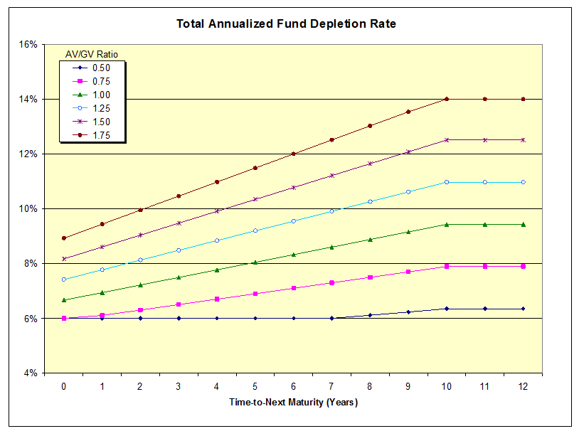
Insurers' capital requirements are set at a supervisory target level that, based on expert judgment, aims to align with a conditional tail expectation (CTE) of 99% over a one-year time horizon including a terminal provision. The risk capital requirements in this guideline are used to compute capital requirements at the target level. An insurer's Base Solvency Buffer (q.v. section 11.3) is calculated in respect of all of its assets, all written insurance business^{Footnote 2}, and all other liabilities. It is equal to the sum of the aggregate capital requirement net of credits, for each of six geographic regions, multiplied by a scalar of 1.0. An aggregate capital requirement is calculated for: Canada The United States The United Kingdom Europe other than the United Kingdom Japan Other locations The aggregate capital requirement within a geographic region comprises requirements for each of the following five risk components: credit risk (Chapters 3 and 4); market risk (Chapter 5); insurance risk (Chapter 6); segregated funds guarantee risk (Chapter 7); and operational risk (Chapter 8). The geographic regions to which an insurer's assets and liabilities are allocated vary with the risk component being calculated: For credit risk and all market risks other than currency risk, all on- and off-balance sheet assets and all liabilities are allocated to the geographic region in which they are currently held, with the exception of: reinsurance contracts that are assets, assets that are pledged as collateral for reinsurance contracts issued, and synthetic asset exposures arising from reinsurance contracts issued (qq.v. sections 3.1.11 and 5.2.3). If an asset or liability is held in a branch, the region in which it is held is deemed to be the region in which the branch is registered. Otherwise, the region in which an asset or liability is held is deemed to be the region in which the legal entity holding the asset or liability is incorporated. The exceptions listed above are allocated to the same geographic regions as those of the corresponding insurance liabilities. For currency risk, the allocation of the requirement to geographic regions is described in section 5.6.7. For insurance risk, segregated fund guarantee risk, and operational risk, liabilities and all of their associated risks are allocated to the geographic regions in which the original policies underlying the liabilities were written directly. Aggregate requirements are reduced by credits for qualifying in-force participating and adjustable products (Chapter 9), and risk diversification (Chapter 11). Additionally, it is possible to obtain credit (via a reduction of specific risk components or an amount recognized in Eligible Deposits) for the following risk mitigation arrangements: reinsurance (insurance risk components, and other components where reinsurance is explicitly recognized); collateral, guarantees and credit derivatives (credit risk component for fixed-income and reinsurance contracts held); other derivatives serving as hedges (market risk components); and asset securitization (credit risk component). Any arrangement (including securitization) under which a third party assumes, or agrees to indemnify an insurer for losses arising from insurance risk is treated as reinsurance for capital purposes, and is subject to the requirements in Chapter 10. Collateral, guarantees and credit derivatives may be used to reduce the credit risk requirements for fixed-income financial assets and registered reinsurance contracts held. The conditions for their use and the capital treatment are described in sections 3.2, 3.3 and 10.4.3. Collateral and letters of credit may be used to reduce the deductions from available capital for unregistered reinsurance in section 10.2, subject to the conditions in section 10.3. Derivatives serving as equity hedges may be applied to reduce the market risk requirements for equities, as described in section 5.2.4, and derivatives serving as foreign exchange risk hedges may be applied to reduce the requirement as described in sections 5.6.2 and 5.6.4. Asset securitization may be used to reduce credit risk requirements as provided for in Guideline B-5: Asset Securitization; guarantees providing tranched protection are treated as synthetic securitizations, and fall within the scope of the securitization guideline. Reinsurance that is intended to mitigate credit or market risks associated with a ceding insurer’s on-balance sheet assets (e.g. equity risk, real estate risk), irrespective of whether it mitigates other risks simultaneously, must meet the conditions and follow the capital treatment specified in sections 10.4.3 and 10.4.4 in order for an insurer to reduce the requirements for these risks.

1.1.6. Foreign life insurers^{Footnote 3}

The Life Insurance Margin Adequacy Test (LIMAT) Ratios are designed to measure the adequacy of assets in Canada of foreign insurers. These ratios and their components (Available Margin, Surplus Allowance and Required Margin) are described in Chapter 12, "Life insurers Operating in Canada on a Branch Basis". The LIMAT is only one element in the determination of the required assets that foreign insurers must maintain in Canada. Foreign insurers must also vest assets in Canada pursuant to section 610 of the Insurance Companies Act.

1.2. Minimum and Supervisory Target ratios

OSFI has established a Supervisory Target Total Ratio of 100% and a Supervisory Target Core Ratio of 70%. The Supervisory Targets provide cushions above the minimum requirements, provide a margin for other risks, and facilitate OSFI's early intervention process^{Footnote 4}. The Superintendent may, on a case by case basis, establish alternative targets in consultation with an insurer based on that insurer's individual risk profile. Insurers are required, at minimum, to maintain a Total Ratio of 90% and a Core Ratio of 55%^{Footnote 5}. Insurers should refer to Guideline A4 - Regulatory Capital and Internal Capital Targets for OSFI's definitions and expectations around the Minimum and Supervisory Target ratios and expectations regarding internal capital targets and capital management policies.

1.3. Accounting basis

Unless indicated otherwise, the starting basis for the amounts used in calculating Available Capital, Available Margin, Surplus Allowance, Base Solvency Buffer, Required Margin and any of their components (such as risk adjustments and contractual service margins) are those reported in, or used to calculate the amounts reported in, the insurer’s financial statements and other financial information contained in the Life Quarterly Return and Life Annual Supplement, all of which have been prepared in accordance with Canadian GAAP^{Footnote 6} in conjunction with OSFI instructions and accounting guidelines. Unless indicated otherwise, the contract boundaries used for insurance liability cash flow projections and all other LICAT components should be the same as those used to prepare the insurer’s financial statements. Financial statements and information are required to be adjusted as specified below to determine the carrying amounts that are subject to capital charges or are otherwise used in LICAT calculations. The Canadian GAAP financial statements and information should be restated for LICAT purposes and reported in accordance with the following specifications: Only subsidiaries (whether held directly or indirectly) that carry on a business that an insurer could carry on directly (e.g., life insurance, real estate and ancillary business subsidiaries) are reported on a consolidated basis.^{Footnote 7} Consolidated equity investments in non-life solvency regulated financial corporations^{Footnote 8} that are controlled should be deconsolidated and reported using the equity method of accounting.

1.4. General requirements

1.4.1. Opinion of the Appointed Actuary

The Appointed Actuary is required to sign, on the front page of the LICAT Quarterly Return^{Footnote 9}, an opinion in accordance with the Standards of Practice of the Canadian Institute of Actuaries. The text of the required opinion is: "I have reviewed the calculation of the LICAT Ratios of [Company name] as at [Date]. In my opinion, the calculations of the components of Available Capital, Surplus Allowance, Eligible Deposits and Base Solvency Buffer have been determined in accordance with the Life Insurance Capital Adequacy Test guideline and the components of the calculation requiring discretion were determined using methodologies and judgment appropriate to the circumstances of the company." [Note: For a foreign insurer "LICAT Ratios", "Available Capital" and "Base Solvency Buffer" are replaced by "LIMAT Ratios", "Available Margin" and "Required Margin".] The memorandum that the Appointed Actuary is required to prepare under the Standards of Practice (LICAT Memorandum) to support this certification must be available to OSFI upon request.

1.4.2. Authorized official signature

Each life insurer is required to have an authorized Officer endorse the following statement on the LICAT Quarterly Return: "I confirm that I have read the Life Insurance Capital Adequacy Test guideline and related instructions issued by the Office of the Superintendent of Financial Institutions and that this form is completed in accordance with them." The Officer attesting to the validity of this statement on the LICAT Quarterly Return at year end must be different from the insurer's Appointed Actuary.

1.4.3. Audit requirement

Life insurers are required to retain an Auditor appointed pursuant to section 337 or 633 of the ICA to report on the year-end LICAT Quarterly Return in accordance with the relevant standards for such assurance engagements, as promulgated by the Canadian Auditing and Assurance Standards Board (AASB).

1.4.4. Best Estimate Liabilities, Cash Flows and Assumptions

Best Estimate Liabilities for one or more policies represents the discounted, probability-weighted mean taken over the full range of possible future cash flows for the policies. If the insurance contract liability for the policies is reported using the IFRS 17 general measurement model or variable fee approach, then the Best Estimate Liability for the policies is equal to the reported insurance contract liability minus the sum of the risk adjustment and contractual service margin^{Footnote 10}. If the insurance contract liability for the policies is reported using the IFRS 17 premium allocation approach, then the Best Estimate Liability for the policies is equal to the reported liability for remaining coverage. Best Estimate Cash Flows for one or more policies, which are used in the calculation of capital requirements for insurance risks, is the estimate of future cash flows whose discounted value determines Best Estimate Liabilities. If the estimate of future cash flows consists of multiple cash flow projections, then Best Estimate Cash Flows is the probability-weighted estimate of future cash flows. If an insurance contract liability for one or more policies is reported using the IFRS 17 premium allocation approach, then Best Estimate Cash Flows comprises outflows of projected future reductions in the liability for remaining coverage that will be recognized as insurance revenue, and inflows of projected future premium receipts. Best Estimate Assumptions are the assumptions underlying Best Estimate Cash Flows. If the estimate of future cash flows consists of multiple cash flow projections, then Best Estimate Assumptions comprises all sets of assumptions that are used to determine any of the cash flow projections.

1.4.5. Use of Approximations

Insurers should adhere to the Standards of Practice of the Canadian Institute of Actuaries on materiality and approximations with respect to approximations permitted within the LICAT. All approximations used, along with the vetting completed to measure the effectiveness of approximations, and the steps taken to refine and correct ineffective approximations, should be reported in the LICAT Memorandum. In addition, insurers should adhere to the following specifications: Approximations of LICAT calculations are not permitted if most of the data or information is available from other internal processes and this data or information is used to calculate liabilities for financial statement purposes. For example, if an insurer performs its liability cash flow projections in real time, it should not use in-arrears asset and liability cash flows for LICAT purposes. In this case, approximations for LICAT should only be used if the actual calculation cannot be performed in real time (i.e. it is done in-arrears for valuation)^{Footnote 11}. Insurers should use approximations consistently from quarter to quarter, unless reviews of their effectiveness require a modification to improve accuracy, or an improvement in the insurer's processes renders the approximation unnecessary. The following approximations may be used in the calculation of the relevant LICAT components:^{Footnote 12} Section 2.1.1: For the volatility adjustment for changes in cost of guarantee liabilities included in Gross Tier 1, insurers may approximate the change to the intrinsic value of guarantees over a quarter by calculating the sensitivity of the intrinsic value at the beginning of the quarter, and then estimating the change in the intrinsic value based on actual market movements that have occurred during the quarter. If such an approximation is used, the approximation methodology should be used consistently over the entire period that the adjustment is used, and sensitivities should be updated each quarter to ensure that quarter-end estimates remain appropriate. Sections 2.1.1.5, 2.1.2.6 and 2.2.1.4: Insurers may approximate marginal capital requirements by using quarter-in-arrears data to determine the ratio of the marginal solvency buffer to the standalone solvency buffer, and then multiplying this ratio by the current standalone solvency buffer. Additionally, the marginal requirements in sections 2.1.1.5 and 2.2.1.4 may be approximated using quarter-in-arrears data if the amount of capital held by third-party investors or attributable to non-controlling interests remains well below the applicable limit. Section 2.1.2.9: Policy-by-policy reserves may be calculated with either the time value of guarantees or total cost of guarantees allocated proportionally by face amount. Section 2.1.2.9.2: An insurer may use quarter-in-arrears data to determine the individual and total policy requirements rc vol, rc cat, RC vol, and RC cat. Section 3.1.2: Quarter-in-arrears cash flows may be used to approximate the effective maturities of credit exposures subject to this section. If this approximation is used, an insurer should make appropriate adjustments for significant changes in asset inventory, disposals, maturities, etc. that have occurred since the last quarter-end. In low-interest rate environments where an insurer is using the weighted average approach to calculate the effective maturity of exposures to a connected group, an insurer may apply weights based on market value instead of undiscounted cash flows to the individual exposures. Section 3.1.7: An insurer may estimate the proportions of reinsurance receivables using quarter-in-arrears data. Section 3.1.7: An insurer may approximate reinsurance contract held assets by reinsurer for the purpose of applying the zero floor by using quarter-in-arrears data to determine the percentage of reserves ceded to each reinsurer, and multiplying these percentages by total current ceded liabilities. Section 3.1.8: An insurer may estimate the proportions of balance sheet receivables that have been outstanding less than 60 days and more than 60 days using quarter-in-arrears data. Sections 5.1.2 and 5.1.3: Quarter-in-arrears cash flows, in combination with roll-forwards and true-ups to capture material changes during the quarter, may be used to determine the most adverse scenario and project all cash flows. If such an approximation is used, the insurer should be able to demonstrate that the quarter-in-arrears cash flows were developed from the same data used for financial statement reporting as of the previous quarter. Section 5.1.3.3: Second-order impacts of restating dividends on paid-up additions may be ignored. Section 5.6.1: The maximum amount of the offsetting short position for a currency within a geographic region may be approximated as: 120 % × BCR currency ∑ BCR × BSB where: BCR currency is the basic capital requirement for business denominated in the currency under consideration, defined below; ∑ BCR is the sum of all basic capital requirements for all currencies within the region; BSB is the Base Solvency Buffer for the region, with all requirements for currency risk excluded, the requirement for insurance risk calculated net of all reinsurance, and all credits for within-risk diversification, between-risk diversification, and participating and adjustable products applicable to the aggregated requirements taken into account. The basic capital requirement BCR currency is the sum of the following amounts that are denominated in the currency under consideration: 2.8% of all liabilities; 0.24% of the net amount at risk (i.e. death benefit minus Best Estimate Liability) for term products and other life products that do not have significant cash values; 2.4% of liabilities for: life products that have significant cash values; participating contracts; and accident, health and disability coverage; 4.8% of annuity liabilities; 4.4% of liabilities for GICs, or of notional value for synthetic GICs (e.g. wraps); and 4.8% of guaranteed value for segregated funds. Insurance liabilities, net amounts at risk, and segregated fund guarantee values in the above sum should be based on Best Estimate Assumptions, and should be measured net of all reinsurance. The guaranteed value of segregated funds is defined to be the actuarial present value of all benefits due to policyholders assuming that all account values are zero, and remain at zero for the life of the policies. Sections 6.2.1 and 6.5.1: Insurers may use cash flows with a lag of up to one year when conducting the tests used to determine which products are life supported and death supported, or lapse supported and lapse sensitive^{Footnote 13}. Sections 6.2.2.1: Insurers may use a lag of up to one year when calculating the ratio of the individual life volatility risk component to the following year's expected claims^{Footnote 13}. Sections 6.4.3, 6.4.4, 6.5.3, 6.5.4, and 6.6.1: For the volatility and catastrophe components of morbidity and lapse risks, the shocks applied to Best Estimate Assumptions are for the first year only, and zero thereafter. If an insurer, for example due to software limitations, is unable to apply shocks for partial calendar years, it may instead apply the LICAT insurance risk shock for the remaining portion of the calendar year, and a different shock for the entirety of the following calendar year. The second shock should be equal to the LICAT shock multiplied by the proportion of the current calendar year that has elapsed. For example, if the insurer is preparing a LICAT filing for the end of Q1 20x1, and LICAT specifies an insurance risk shock of 30%, then the insurer may use a shock of 30% for the remainder of 20x1, and a 7.5% shock for all of 20x2. If this approximation is used for expense risk, the second shock representing the carryover from the first year should be added to the 10% shock in the second year. Section 6.5.3: An insurer may approximate the requirement for lapse volatility by determining the present value of cash flows for a shock of +/- 30% in the first year, and subtracting the present value of Best Estimate Cash Flows. Sections 6.8.1, 6.8.4, and 9.2: In order to determine a marginal insurance risk solvency buffer, insurers may use quarter-in-arrears data to determine the ratio of the marginal insurance risk solvency buffer to the standalone insurance risk solvency buffer, and then apply this ratio to the current standalone insurance risk solvency buffer. An insurer may use this approximation if changes from the previous quarter (e.g. diversification credit or the relative weights of different risks) do not have a material impact on the results.

1.5. Minimum amount of Available Capital

Notwithstanding the minimum and target Total and Core Ratios described in the Guideline, Canadian life insurance companies are required to maintain a minimum amount of Available Capital, as calculated in this Guideline, of $5 million or such amount as specified by the Superintendent.

Footnotes

Footnote 1 Surplus Allowance should be reported net of all modified coinsurance, both registered and unregistered. Return to footnote 1 Footnote 2 All future business written is excluded from the calculation of the Base Solvency Buffer. Return to footnote 2 Footnote 3 Within this guideline, the term "foreign life insurer" has the same meaning as life insurance "foreign company" in section 2 of the Insurance Companies Act. Return to footnote 3 Footnote 4 Industry-wide Supervisory Targets are not applicable to regulated insurance holding companies and non-operating insurance companies. Return to footnote 4 Footnote 5 During 2023 and 2024, regulated insurance holding companies and non-operating insurance companies are required to maintain a minimum Core Ratio of 50%. Starting in 2025, the minimum Core Ratio for regulated insurance holding companies and non-operating insurance companies will be 55%. Return to footnote 5 Footnote 6 The Canadian Accounting Standards Board has adopted International Financial Reporting Standards (IFRS) as Canadian GAAP for publicly accountable enterprises, including insurers. The primary source of Canadian GAAP is the Chartered Professional Accountants of Canada Handbook. Return to footnote 6 Footnote 7 Composite insurance subsidiaries that write both life insurance and property and casualty insurance are included within the scope of consolidation. Composite insurance subsidiaries are subject to all of the requirements of this guideline for credit, market and operational risks and, with the exception property and casualty insurance liabilities (q.v. section 6.7), insurance risk. Return to footnote 7 Footnote 8 Non-life solvency regulated financial corporations include entities engaged in the business of banking, trust and loan business, property and casualty insurance business, the business of cooperative credit societies or that are primarily engaged in the business of dealing in securities, including portfolio management and investment counselling. Return to footnote 8 Footnote 9 The Appointed Actuary is only required to sign the front page of the LICAT Quarterly Return for submissions made at year end. Return to footnote 9 Footnote 10 For participating policies, the Best Estimate Liability excludes all liability accounts that are recognized within Available Capital. Return to footnote 10 Footnote 11 Approximations 8 and 9 below may be used notwithstanding this condition. Return to footnote 11 Footnote 12 Only the approximations listed below may be used for LICAT components that affect the LICAT ratios materially. Other immaterial approximations may be used in the determination of the LICAT ratios. Return to footnote 12 Footnote 13 During 2023, an insurer may base the approximation on cash flows that were determined during 2022 under the accounting standards that existed prior to the adoption of IFRS 17 if cash flows under IFRS 17 are not readily available. Return to footnote 13

This chapter defines the elements included in Available Capital, establishes criteria for assessing capital instruments, and sets capital composition limits. The primary considerations for assessing the capital elements of an insurer include: availability: whether the capital element is fully paid in, and the extent to which it is available to absorb losses; permanence: the period for which the capital element is available to absorb losses; absence of encumbrances and mandatory servicing costs: the extent to which the capital element is free from mandatory payments or encumbrances; and subordination: the extent to, and the circumstances under which the capital element is subordinated to the rights of policyholders and general creditors of the insurer in an insolvency or winding-up. Total available capital comprises Tier 1 and Tier 2 capital, which are defined in sections 2.1 and 2.2 below.

2.1. Tier 1

2.1.1. Gross Tier 1

Gross Tier 1 is equal to the sum of:

Tier 1 Capital Instruments

Common shares issued by the insurer, other than those issued by consolidated subsidiaries and held by third party investors, that meet the criteria specified in section 2.1.1.1; Tier 1 Capital Instruments other than Common Shares issued by the insurer, other than those issued by consolidated subsidiaries and held by third party investors: that meet the criteria specified in sections 2.1.1.2 to 2.1.1.4; or that were issued prior to August 7, 2014, do not meet the criteria specified in sections 2.1.1.2 to 2.1.1.4, but meet the Tier 1 criteria specified in Appendix 2-B and Appendix 2-C of the OSFI guideline Minimum Continuing Capital and Surplus Requirements effective January 1, 2016 (these instruments are subject to the transition measures in section 2.4.1); Instruments issued by consolidated subsidiaries of the insurer and held by third party investors: that meet the criteria for classification as Common Shares as specified in section 2.1.1.1, or as Tier 1 Capital Instruments other than Common Shares as specified in sections 2.1.1.2 to 2.1.1.4 (these instruments are subject to the conditions in section 2.1.1.5 and the transition measures in section 2.4.2); or that were issued prior to August 7, 2014, do not meet the criteria specified in sections 2.1.1.2 to 2.1.1.4, but meet the Tier 1 criteria specified in Appendix 2-B and Appendix 2-C of the OSFI guideline Minimum Continuing Capital and Surplus Requirements effective January 1, 2016 (these instruments are subject to transition measures in sections 2.4.1 and 2.4.2).

Tier 1 Elements other than Capital Instruments

Contributed Surplus, comprising: Share premium resulting from the issuance of capital instruments included in Gross Tier 1^{Footnote 1}; and Other contributed surplus, resulting from sources other than profits (e.g., members' contributions and initial funds for mutual companies and other contributions by shareholders in excess of amounts allocated to share capital for joint stock companies), excluding any share premium resulting from the issuance of capital instruments included in Tier 2; Adjusted Retained Earnings; Volatility adjustment for changes in cost of guarantee liabilities: An insurer may, at its option and for a limited period of seven quarters, partially reverse changes that have occurred in the liability for the cost of guarantees for participating and non-participating products (excluding segregated funds) since the end of the previous quarter. A one-time election of whether to use this option must be made within three months after the adoption of IFRS 17, and cannot be changed thereafter. If the insurer elects to use the adjustment, then starting after the first quarter end at which IFRS 17 is used for reporting, a percentage of the increase (decrease) in the liability for cost of guarantees caused by market movements is added to (subtracted from) Gross Tier 1, where the increase or decrease is measured from the end of the previous quarter to the reporting date^{Footnote 2}. For reporting dates within the first year after the adoption of IFRS 17, the percentage used for the adjustment is 50%, and for the second year after the adoption of IFRS 17, the percentage used is 25%. Market movements include changes to risk-free interest rates, equity prices, and credit spreads. Insurers may use their own internal processes to determine the portion of the change in liability for cost of guarantees that has occurred due to market movements. The liability for cost of guarantees to which the partial reversal is applied comprises the liabilities for both the intrinsic value of the guarantees, and the time value of the guarantees. Adjusted Accumulated Other Comprehensive Income (AOCI); Participating account^{Footnote 3}; Non-participating account (mutual companies)^{Footnote 4}; Tier 1 elements, other than capital instruments, attributable to non-controlling interests that satisfy the conditions in section 2.1.1.5; and Tax adjustments and amounts recoverable on surrender related to policy-by-policy negative reserves ceded under unregistered reinsurance (qq.v. sections 10.2.5 and 10.2.6). To determine Adjusted Retained Earnings, the following adjustments are made to retained earnings^{Footnote 5}: All contractual service margins that are reported as liabilities in the financial statements^{Footnote 6}, other than those in respect of segregated fund contracts with guarantee risks, are added; All contractual service margins that are reported as assets in the financial statements^{Footnote 6}, other than those in respect of segregated fund contracts with guarantee risks, are subtracted; The impact of accumulated after-tax gains or losses on fair-valued liabilities arising from changes to the insurer's own credit risk is reversed; The impact of the following items related to real estate is reversed: After-tax fair value gains or losses on owner-occupied property upon conversion to IFRS (cost model)^{Footnote 7}; Accumulated after-tax revaluation loss on owner-occupied property (revaluation model); Gains or losses up to the transfer date on owner-occupied property that was previously classified as investment property^{Footnote 8}; The impact of any discretionary participation features reported in a component of equity that is included in Gross Tier 1 is reversed. To determine Adjusted AOCI, the following adjustments are made to total reported AOCI: The impact of accumulated after-tax gains or losses on fair-valued liabilities arising from changes to the insurer’s own credit risk is reversed; The impact of /accumulated fair value gains and losses on derivatives held as cash flow hedges relating to the hedging of items that are not fair-valued on the balance sheet (e.g., loans and debt obligations) is reversed; and Accumulated after-tax fair value revaluation gains on own-use property under the revaluation method are subtracted.

2.1.1.1 Qualifying Criteria for Common Shares

Capital instruments classified as common shares must meet all of the following criteria: The shares represent the most subordinated claim in liquidation of the insurer. The investor is entitled to a claim on the residual assets that is proportional with its share of issued capital, after all senior claims have been paid in liquidation (i.e., has an unlimited and variable claim, not a fixed or capped claim). The principal is perpetual and never repaid outside of liquidation (setting aside discretionary repurchases or other means of effectively reducing capital in a discretionary manner that are allowable under relevant law and subject to the prior approval of the Superintendent). The insurer does not, in the sale or marketing of the instrument, create an expectation at issuance that the instrument will be bought back, redeemed or cancelled, nor do the statutory or contractual terms provide any feature that might give rise to such expectation. Distributions are paid out of distributable items (retained earnings included). The level of distributions is not in any way tied or linked to the amount paid in at issuance, and is not subject to a contractual cap (except to the extent that an insurer is unable to pay distributions that exceed the level of distributable items or to the extent that distributions on senior ranking capital must be paid first). There are no circumstances under which the distributions are obligatory. Non-payment is therefore not an event of default. Distributions are paid only after all legal and contractual obligations have been met and payments on more senior capital instruments have been made. This means that there are no preferential distributions, including in respect of other elements classified as the highest quality issued capital. It is in the form of issued capital that takes the first and proportionately greatest share of any losses as they occur. Within the highest quality capital, each instrument absorbs losses on a going-concern basis proportionately and pari passu with all the others. The paid-in amount is recognized as equity capital (i.e., not recognized as a liability) for determining balance sheet solvency. It is directly issued and paid-in^{Footnote 9} and the insurer cannot directly or indirectly have funded the purchase of the instrument. Where the consideration for the shares is given in a form other than cash, the issuance of the common shares is subject to the prior approval of the Superintendent. The paid-in amount is neither secured nor covered by a guarantee of the issuer or a related entity^{Footnote 10}, and is not subject to any other arrangement that legally or economically enhances the seniority of the claim. It is only issued with the approval of the owners of the issuing insurer, either given directly by the owners or, if permitted by applicable law, given by the Board of Directors or by other persons duly authorised by the owners. It is clearly and separately disclosed as equity on the insurer's balance sheet, prepared in accordance with relevant accounting standards. The criteria for common shares also apply to instruments issued by non-joint stock companies, such as mutual insurance companies and fraternal benefit societies, taking into account their specific constitutions and legal structures. The application of the criteria should preserve the quality of the instruments by requiring that they be deemed fully equivalent to common shares in terms of their capital quality, including their loss absorption capacity, and do not possess features that could cause the condition of the insurer to be weakened as a going concern during periods when the insurer is under stress.

2.1.1.2 Qualifying Criteria for Tier 1 Capital Instruments Other than Common Shares^{Footnote 11}

Instruments, other than common shares, qualify as Tier 1 if all of the following criteria are met: The instrument is issued and paid-in in cash or, subject to the prior approval of the Superintendent, in property. The instrument is subordinated to policyholders, general creditors, and subordinated debt holders of the insurer. The instrument is neither secured nor covered by a guarantee made by the issuer or a related entity, and there is no other arrangement that legally or economically enhances the seniority of the claim vis-à-vis the insurer's policyholders and general creditors^{Footnote 12}. The instrument is perpetual, i.e., there is no maturity date, and there are no step-ups^{Footnote 13} or other incentives to redeem^{Footnote 14}. The instrument may be callable at the initiative of the issuer only after a minimum of five years: To exercise a call option an insurer must receive prior approval of the Superintendent; and An insurer's actions and the terms of the instrument must not create an expectation that the call will be exercised; and An insurer must not exercise the call unless: It replaces the called instrument with capital of the same or better quality, including through an increase in retained earnings, and the replacement of this capital is made on terms that are sustainable for the income capacity of the insurer^{Footnote 15}; or The insurer demonstrates that its capital position is well above the supervisory target capital requirements after the call option is exercised^{Footnote 16}. Any repayment of principal (e.g. through repurchase or redemption) requires Superintendent approval and insurers must not assume or create market expectations that such approval will be given. Dividend / coupon discretion: The insurer must have full discretion at all times to cancel distributions/ payments^{Footnote 17}. Cancellation of discretionary payments must not be an event of default or credit event. Insurers must have full access to cancelled payments to meet obligations as they fall due. Cancellation of distributions/payments must not impose restrictions on the insurer except in relation to distributions to common shareholders. Dividends/coupons must be paid out of distributable items. The instrument cannot have a credit sensitive dividend feature, i.e., a dividend/coupon that is reset periodically based in whole or in part on the insurer's credit standing^{Footnote 18}. The instrument cannot contribute to liabilities exceeding assets if such a balance sheet test forms part of insolvency law. Other than preferred shares, instruments included in Tier 1 Capital must be classified as equity per relevant accounting standards. Neither the insurer nor a related party over which the insurer exercises control or significant influence can have purchased the instrument, nor can the insurer directly or indirectly have funded the purchase of the instrument. The instrument cannot have any features that hinder recapitalisation, such as provisions that require the issuer to compensate investors if a new instrument is issued at a lower price during a specified timeframe. If the instrument is not issued out of an operating entity or the holding company in the consolidated group (e.g. it is issued out of a special purpose vehicle (SPV)), proceeds must be immediately available without limitation to an operating entity^{Footnote 19} or the holding company in the consolidated group in a form which meets or exceeds all of the other criteria for inclusion in Tier 1^{Footnote 20}. Purchase for cancellation of Tier 1 Capital instruments Other than Common Shares is permitted at any time with the prior approval of the Superintendent. For further clarity, a purchase for cancellation does not constitute a call option as described in the above qualifying criteria. Tax and regulatory event calls are permitted during an instrument’s life subject to the prior approval of the Superintendent, and provided the insurer was not in a position to anticipate such an event at the time of issuance. Where an insurer elects to include a regulatory event call in an instrument, the regulatory event call date should be defined as “the date specified in a letter from the Superintendent to the Company on which the instrument will no longer be recognized in full as eligible Tier 1 capital of the insurer on a consolidated basis”. Dividend stopper arrangements that stop payments on Common Shares or Tier 1 Capital Instruments Other than Common Shares are permissible provided the stopper does not impede the full discretion the insurer must have at all times to cancel distributions or dividends on the Tier 1 Capital Instrument Other than Common Shares, nor must it act in a way that could hinder the recapitalization of the insurer pursuant to criterion # 13 above. For example, it would not be permitted for a stopper on Tier 1 Capital Instruments Other than Common Shares to: attempt to stop payment on another instrument where the payments on the other instrument were not also fully discretionary; prevent distributions to shareholders for a period that extends beyond the point in time that dividends or distributions on the Tier 1 Capital Instruments Other than Common Shares are resumed; or impede the normal operation of the insurer or any restructuring activity, including acquisitions or disposals. A dividend stopper may also act to prohibit actions that are equivalent to the payment of a dividend, such as the insurer undertaking discretionary share buybacks. Where an amendment or variance of a Tier 1 instrument’s terms and conditions affects its recognition as Available Capital, such an amendment or variance will only be permitted with the prior approval of the Superintendent^{Footnote 21}. An insurer is permitted to "re-open" offerings of capital instruments to increase the principal amount of the original issuance subject to the following: the insurer may not re-open an offering if the initial issue date for the offering was on or before August 7, 2014 and the offering does not meet the criteria in section 2.1.1.2; and call options may only be exercised, with the prior approval of the Superintendent, on or after the fifth anniversary of the closing date of the latest re-opened tranche of securities. Defeasance options may only be exercised on or after the fifth anniversary of the closing date with the prior approval of the Superintendent.

2.1.1.3 Tier 1 Capital Instruments Other than Common Shares issued to a Parent

In addition to the qualifying criteria and minimum requirements specified in this Guideline, Tier 1 Capital Instruments Other than Common Shares issued by an insurer to a parent, either directly or indirectly, can be included in Available Capital subject to the insurer providing prior written notification of the intercompany issuance to OSFI’s Capital Division, together with the following: a copy of the instrument's terms and conditions; the intended classification of the instrument for Available Capital purposes; the rationale for not issuing common shares in lieu of the subject capital instrument; confirmation that the rate and terms of the instrument are at least as favourable to the insurer as market terms and conditions; confirmation that the failure to make dividend or interest payments, as applicable, on the subject instrument would neither result in the parent, now or in the future, being unable to meet its own debt servicing obligations, nor would it trigger cross-default clauses or credit events under the terms of any agreements or contracts of either the insurer or the parent.

2.1.1.4 Tier 1 Capital Instruments Other than Common Shares issued out of Branches and Subsidiaries outside Canada

In addition to any other requirements prescribed in this Guideline, where an insurer wishes to include, in its consolidated Available Capital, Tier 1 Capital Instruments Other than Common Shares issued out of a branch or subsidiary of the insurer outside Canada, it should provide OSFI’s Capital Division with the following documentation: a copy of the instrument's terms and conditions; certification from a senior executive of the insurer, together with the insurer's supporting analysis, that confirms that the instrument meets the qualifying criteria for the tier of Available Capital in which the insurer intends to include the instrument on a consolidated basis; and an undertaking whereby both the insurer and the subsidiary confirm that the instrument will not be redeemed, purchased for cancellation, or amended without the prior approval of the Superintendent. Such an undertaking will not be required where the prior approval of the Superintendent is incorporated into the terms and conditions of the instrument.

2.1.1.5 Consolidated Subsidiaries having Tier 1 Third Party Investors / Non-Controlling Interests

Both: Common Shares, and Tier 1 Capital Instruments other than Common Shares, issued by a consolidated subsidiary of the insurer and held by third party investors, and Tier 1 elements, other than capital instruments, attributable to non-controlling interests^{Footnote 22} are subject to limited recognition in the consolidated Tier 1 capital of the parent insurer^{Footnote 23}. Tier 1 capital instruments issued by a subsidiary and held by third party investors are included in consolidated Tier 1 capital if: They are issued for the funding of the parent insurer and meet all of the following criteria: The subsidiary uses the proceeds of the issue to purchase a similar instrument from the parent insurer that meets the criteria in section 2.1.1.1, or sections 2.1.1.2 to 2.1.1.4; The terms and conditions of the issue, as well as the intercompany transfer, place the investors in the same position as if the instrument were issued by the parent insurer; and The instrument held by third party investors is not effectively secured by other assets, such as cash, held by the subsidiary. or: They were issued prior to September 13, 2016 and qualify for recognition in consolidated Available Capital under section 2.4.2. Tier 1 capital instruments issued by a subsidiary and held by third party investors that do not meet the above criteria, and Tier 1 elements, other than capital instruments, attributable to non-controlling interests, may be included in the consolidated Tier 1 capital of the parent insurer subject to the following Third Party Share limit: Third Party Share Percentage × (Marginal capital requirement for the subsidiary + Total deductions from the subsidiary's Available Capital) where: Third Party Share Percentage is equal to the total amount of all Tier 1 and Tier 2 capital instruments issued by a subsidiary and held by third party investors that do not meet the above criteria, plus Tier 1 elements, other than capital instruments, attributable to non-controlling interests^{Footnote 22}, divided by the sum of Available Capital and the Surplus Allowance of the subsidiary. Marginal capital requirement for the subsidiary^{Footnote 2} is equal to: the difference between the Base Solvency Buffer (q.v. section 11.3) of the insurer, and the Base Solvency Buffer of the insurer excluding the subsidiary, with both requirements calculated net of all reinsurance, if the sum of Tier 1 and Tier 2 capital instruments issued by a subsidiary and held by third parties and of Tier 1 elements, other than capital instruments, attributable to non-controlling interests is equal to or greater than 1% of Gross Tier 1, or the capital requirement of the subsidiary calculated based on local regulatory requirements at the equivalent local level of the LICAT supervisory target,^{Footnote 24} if the sum of Tier 1 and Tier 2 capital instruments issued by a subsidiary and held by third parties and Tier 1 elements, other than capital instruments, attributable to non-controlling interests is less than 1% of Gross Tier 1.

2.1.2. Deductions from Gross Tier 1 Capital

The items below are deducted from Gross Tier 1 to determine Net Tier 1. Credit risk factors are not applied to items that are deducted from Gross Tier 1.

2.1.2.1. Goodwill and other intangible assets

Goodwill related to consolidated subsidiaries^{Footnote 25} and goodwill included in the carrying amount of equity accounted substantial investments^{Footnote 26} is deducted from Gross Tier 1. The amount deducted is net of any associated deferred tax liabilities (DTLs) that would be extinguished if the goodwill were to become impaired or otherwise derecognized. Additionally, all other intangible assets (including software intangibles) are deducted from Gross Tier 1, including intangible assets related to consolidated subsidiaries and intangible assets included in the carrying amount of equity-accounted substantial investments. The amount deducted is net of any associated DTLs that would be extinguished if the intangible assets were to become impaired or otherwise derecognized.

2.1.2.2. Investments in own Tier 1 Capital

An insurer's investments in its own common shares (e.g. treasury stock) and its own Tier 1 Capital Instruments other than Common Shares, whether held directly or indirectly, are deducted from Gross Tier 1 unless they are already derecognized under IFRS. In addition, any Tier 1 capital instrument that the insurer could be contractually obliged to purchase is deducted from Gross Tier 1.

2.1.2.3. Reciprocal Cross Holdings of Tier 1 Capital of banking, insurance and financial entities

Reciprocal cross holdings in Tier 1 capital instruments (e.g. Insurer A holds investments in Tier 1 capital instruments of Insurer B, and in return, Insurer B holds investments in Tier 1 capital instruments of Insurer A), whether arranged directly or indirectly, that are designed to artificially inflate the capital position of insurers are deducted from Gross Tier 1.

2.1.2.4. Net Defined Benefit Pension Plan Assets

Each net defined benefit pension plan asset (DB pension plan), inclusive of the impact of any asset ceiling limitation, is deducted from Gross Tier 1, net of any associated DTLs that would be extinguished if the asset were to become impaired or derecognized^{Footnote 27}. An insurer may reduce this deduction by the amount of available refunds of surplus assets in the plan to which the insurer has unrestricted and unfettered access, provided it obtains prior written OSFI supervisory approval^{Footnote 28}.

2.1.2.5. Deferred tax assets

The regulatory adjustments described in this section are based on non-discounted deferred tax amounts as reported on the insurer's balance sheet, and on the deferred tax position of each legal entity that is consolidated for LICAT purposes. Deferred tax assets (DTA) must be classified as either DTA arising from temporary differences (DTA Temporary) or DTA other than those arising from temporary differences (DTA Non-Temporary). For example, DTA relating to tax credits and DTA relating to carry forwards of operating losses are classified as DTA Non-Temporary. No regulatory adjustments are required under this section for legal entities in a net Deferred Tax Liability (DTL) position. Regulatory adjustments associated with legal entities in net DTA positions are set out in sections 2.1.2.5.1 and 2.1.2.5.2 below. Eligible DTL, in this section, are limited to those permitted to offset DTA for balance sheet reporting purposes at the legal entity level, excluding DTL that have been netted against the deductions for goodwill, intangible assets and defined benefit pension plan assets. Eligible DTL are allocated on a pro rata basis between DTA Temporary and DTA Non-Temporary. 2.1.2.5.1 DTA – other than those arising from temporary differences Insurers should deduct 100% of DTA Non-Temporary, net of eligible DTL, from Gross Tier 1. 2.1.2.5.2 DTA – arising from temporary differences The amount that insurers should deduct from Gross Tier 1 is: max DTAT net − 0.1 × T 1 gross − T 1 deductions , 0 0.9 where: DTAT net is equal to DTA Temporary net of eligible DTL T1 gross is equal to Gross Tier 1 T1 deductions is equal to the sum of all deductions from Gross Tier 1 in sections 2.1.2.1 to 2.1.2.5.1, and sections 2.1.2.6 to 2.1.2.10. DTA Temporary included in Available Capital is limited to 10% of Net Tier 1, and is subject to a 25% credit risk factor (q.v. section 3.1.8). The following is an example for a single legal entity reporting LICAT results: Example: Deferred Tax Assets Item Amount Gross Tier 1 4,075 All deductions from Gross Tier 1 except those relating to both types of DTA 2,000 DTA Non-Temporary 100 DTA Temporary 300 DTL associated with goodwill 50 DTL other 100 Net DTA position (100 + 300 - 50 - 100) = 250 DTL allocated to DTA Non-Temporary 100 400 × 100 = 25 (excludes DTL associated with goodwill) DTL allocated to DTA Temporary 300 400 × 100 = 75 (excludes DTL associated with goodwill) DTA Non-Temporary, net of eligible DTL 100 - 25 = 75 DTA Temporary, net of eligible DTL 300 - 75 = 225 Gross Tier 1, net of 2.1.2.1 to 2.1.2.5.1 and 2.1.2.6 to 2.1.2.10 deductions 4,075 - 2,000 - 75 = 2,000 DTA deducted from Gross Tier 1 1) 75 (DTA Non-Temporary) 2) 225 − ( 10% × 2000 ) 0.9 = 28 ( DTA Temporary ) Validation: Amount included in Available Capital does not exceed 10% of Tier 1 2,000 - 28 = 1,972 197 / 1,972 = 10% Capital charged on DTA Temporary included in Available Capital (250 + 50) - (75 + 28) = 197 × 25% = 49

2.1.2.6. Encumbered Assets

Encumbered assets in excess of the allowable amount are deducted from Gross Tier 1^{Footnote 29}. The allowable amount, which is calculated for each pool of encumbered assets and the liabilities they secure^{Footnote 30}, is equal to the sum of: the value of on-balance sheet liabilities secured by the encumbered assets; and the marginal capital requirement^{Footnote 2}, floored at zero, for the encumbered assets and the liabilities they secure. The deduction is reduced by the following amount: 50% of the calculated deduction amount relating to real property pledged to secure mortgage borrowing activities. For the purpose of calculating the allowable amount, the marginal capital requirement is equal to the difference between the Base Solvency Buffer (q.v. section 11.3) of the insurer, and the Base Solvency Buffer of the insurer excluding the encumbered assets and the liabilities they secure^{Footnote 31}, where both requirements are calculated net of all reinsurance. The balance sheet amount of liabilities secured by encumbered assets not in excess of the allowable amount and not deducted from Available Capital is subject to section 3.5 of this guideline. The following encumbered assets are exempt and should not be included in the calculation of the encumbered assets deduction above: assets relating to off-balance sheet securities financing transactions (i.e., securities lending and borrowing, repos and reverse repos) that do not give rise to any liability on the balance sheet; and assets pledged to secure centrally cleared and non-centrally cleared derivatives liabilities. Encumbered assets relating to off-balance sheet securities financing transactions that are exempt under 1) above are subject to section 3.5 of this guideline.

2.1.2.7. Investments in Tier 1 Capital of controlled non-life financial corporations

Investments in financial instruments of controlled (as defined in the Insurance Companies Act) non-life solvency regulated financial corporations are deducted^{Footnote 32} from the tier of capital for which the instrument would qualify if it were issued by the insurer itself. Where an instrument issued by a controlled non-life financial corporation meets the criteria outlined in section 2.1.1.1 or 2.1.1.2, it is deducted from Gross Tier 1. If the instrument in which the insurer has invested does not meet the qualifying criteria for either Tier 1 or Tier 2, the instrument is deducted from Gross Tier 1. The amount deducted is the carrying amount of the deconsolidated subsidiary reported as an investment using the equity method of accounting, as specified in section 1.3. The deduction of this amount therefore includes the goodwill, all other intangible assets, net DB pension plan assets, DTAs, encumbered assets, AOCI and all other net assets of the deconsolidated subsidiary, as the de-consolidation should reverse these amounts prior to their respective Gross Tier 1 deductions. Where the insurer provides a facility such as a letter of credit or guarantee that is treated as capital^{Footnote 33} by the controlled non-life financial corporation, the full amount of the facility is deducted from Gross Tier 1^{Footnote 34}. A credit risk factor will not be applied to equity investments, letters of credit and guarantees or other facilities provided to controlled non-life financial corporations where these have been deducted from Available Capital. Where letters of credit or guarantees are provided to controlled non-life financial corporations and are not deducted from Available Capital, they are treated as direct credit substitutes in accordance with this guideline (refer to Chapters 3 and 4).

2.1.2.8. Cash surrender value deficiencies calculated by aggregated sets

Cash surrender value (CSV) deficiencies are calculated net of all reinsurance on an aggregate basis within sets by product type. Deficiencies are calculated relative to fulfillment cash flows. The deduction from Gross Tier 1 is the sum of the positive deficiencies taken over each set of policies, where the positive deficiency for a set is the higher of the set’s aggregate deficiency or zero. All of the policies in an aggregated set must be within the same line of business (as defined in the LIFE return), must be contractually similar, and must eventually offer a meaningful cash surrender value. Policies that never pay CSVs may not be used to offset deficiencies in policies that do. The CSVs used in the calculation of deficiencies should be net of all surrender charges, market value adjustments and other deductions that an insurer could reasonably expect to apply in the event the policy were to be surrendered.

2.1.2.9. Negative reserves and deferred acquisition costs calculated policy-by-policy

In this section, policy-by-policy negative reserves are defined to be negative Best Estimate Liabilities calculated on a policy-by-policy basis. Insurers should calculate policy-by-policy negative reserves net of all reinsurance^{Footnote 35}. Policy-by-policy negative reserves are reduced by a percentage factor of either 10% or 30%, and then reduced further for amounts that may be recovered on surrender. The deduction from Gross Tier 1 or the amount included in Assets Required is the total amount, calculated policy-by-policy, of negative reserves net of reductions, with the net amount for each policy subject to a minimum of zero. Policy-by-policy negative reserves should be calculated for all products and lines of business, including group and accident and sickness business, and future business assumed through reinsurance contracts issued^{Footnote 2}. The calculation should include: the negative reserve for each certificate under group insurance policies for which premiums or reserves are based on individual insured characteristics, such as group association or creditor insurance; the excess, if positive, of the deferred acquisition costs for any policy (including deferred acquisition costs for policies for which coverage has not yet become effective) over its termination or surrender charges; and negative group insurance refund provisions where recovery is not completely assured, calculated policy by policy. The negative reserve for any policy may be reduced by 10%. In order to account for the effect of income taxes, the negative reserve for a policy may be reduced by an additional 20% of the original negative reserve amount if it arises from either of the following: active life reserves for individually underwritten Canadian health business, or Individually underwritten Canadian life business. No reduction for the effect of income taxes is made to negative reserves relating to any other type of business. The negative reserve may then be further reduced, to a minimum of zero, by the sum of the following amounts recoverable on surrender: 85% of the net commission chargeback for the policy; The product of γ , 1 + f , and 70% of the policy's marginal insurance risk requirement, where γ is the scalar defined in section 1.1.5, and f is the operational risk factor applied to required capital for insurance risk in section 8.2.3^{Footnote 36}; a specified amount if the policy is part of a yearly renewable term (YRT) reinsurance treaty; and outstanding earned premiums for group insurance business. However, the maximum total amount by which the deduction from Gross Tier 1 of reduced policy-by-policy negative reserves for a Canadian insurer may be further reduced for amounts recoverable on surrender is limited to 130% of: Gross Tier 1; plus 70% of Surplus Allowance; less All deductions from Gross Tier 1 used to determine Net Tier 1 as specified in section 2.1.2, excluding negative reserves and adjustments for unregistered reinsurance; less Total policy-by-policy negative reserves reduced by percentage factors, but not by any amounts recoverable on surrender; less The deductions from Tier 1 for unregistered reinsurance in sections 10.2.1 to 10.2.4, net of any credits applicable in sections 10.2.1 and 10.2.2; plus The addition to Tier 1 in section 10.2.5. For a foreign insurer, the maximum amount by which reduced policy-by-policy negative reserves included in Assets Required may be further reduced for amounts recoverable on surrender is limited to 130% of: admitted assets vested in trust; plus investment income due and accrued on admitted vested assets; plus 70% of Surplus Allowance; less Deductions/Adjustments (q.v. section 12.2.4); less Assets Required (q.v. section 12.2.5) excluding negative reserves in item 10) and amounts recoverable on surrender in item 21); less total policy-by-policy negative reserves reduced by percentage factors, but not by any amounts recoverable on surrender. If the amount by which policy-by-policy negative reserves is reduced for amounts recoverable on surrender is below the applicable limit, then the difference may be allocated among unregistered reinsurers to increase the corresponding limits in the unregistered reinsurance adjustments for amounts recoverable on surrender (q.v. section 10.2.6). In order to use any amount recoverable on surrender to offset a policy's negative reserve, the amount must be calculated for that policy alone. The following provides additional detail on the calculation of each amount. 2.1.2.9.1. Commission chargebacks The net commission chargeback for a policy is equal to S × C , where: S is 70% if the policy’s negative reserve has been reduced by 20% to account for the effect of income taxes, and is 100% if it has not; and C is the policy’s commission chargeback that the insurer could reasonably expect to recover in the event the policy were to lapse. The chargeback amount used should be based on the policy’s chargeback schedule, and should be calculated net of all ceded reinsurance allowances and commissions. 2.1.2.9.2. Marginal insurance risk requirements The marginal insurance risk requirement for a policy is equal to the sum of the marginal policy requirements for each of the seven insurance risks as specified below. In determining the offset to a policy’s reduced negative reserve, the policy’s marginal insurance risk requirement should be reduced by the amount of any credits that an insurer has taken on account of policyholder deposits and group business adjustments (qq.v. sections 6.8.2 and 6.8.3). Each marginal policy requirement should be calculated net of all reinsurance. All marginal policy requirements for qualifying participating and adjustable products should be multiplied by 30%. The negative reserve for a policy may not be offset by any marginal insurance risk component if an insurer has taken a reduction in required capital on account of a reinsurance claims fluctuation reserve covering the policy. For a policy within a specific geographic region, the marginal policy requirement for mortality risk is equal to: 0.4×rcvol2+2×rccat×RCcat-rccat2RCvol2+RCcat2+0.9×(rcl+rct) where^{Footnote 2}: rcvol is the mortality volatility risk component for the policy rccat is the mortality catastrophe risk component for the policy RCvol is the mortality volatility risk component for all business in the policy's geographic region RCcat is the mortality catastrophe risk component for all business in the policy's geographic region rcl is the policy's level component for mortality risk rct is the policy's trend component for mortality risk The marginal policy requirement for expense risk is equal to 90% of the policy's total requirement for the risk. For all other insurance risks, the marginal policy requirement is equal to: 0.4 × 2 × rc vol × RC vol + 2 × rc cat × RC cat − rc vol 2 − rc cat 2 RC vol 2 + RC cat 2 + 0.9 × ( rc l + rc t ) where^{Footnote 2}: rcvol is the volatility component of the particular insurance risk for the policy (multiplied by the statistical fluctuation factor of the policy's geographic region if applicable) rccat is the catastrophe component of the particular insurance risk for the policy RCvol is the volatility component of the particular insurance risk for all business in the policy's geographic region RCcat is the catastrophe component of the particular insurance risk for all business in the geographic region rcl is the policy's level component for the particular insurance risk, multiplied by the statistical fluctuation factor of the policy's geographic region if applicable rct is the policy's trend component for the particular insurance risk 2.1.2.9.3. Policies assumed under YRT treaties If a policy has been assumed under an eligible YRT reinsurance treaty (defined as a treaty that has fully guaranteed premiums and does not provide for profit sharing), the adjustment that may be used to reduce the policy's negative reserve is: NR × min A − B A , 0.25 where: NR is the policy’s negative reserve reduced by percentage factors; A is the total of reduced negative reserves for all policies within the insurer’s eligible YRT reinsurance treaties calculated policy-by-policy; and B is the total of reduced negative reserves for all of the insurer’s eligible YRT reinsurance treaties, calculated treaty by treaty. 2.1.2.9.4 Outstanding earned premiums for group insurance business If all premiums due under a group insurance policy are an obligation of the plan sponsor, an amount recoverable on surrender for outstanding earned premiums on the policy may be recognized. The outstanding earned premium for the policy is defined to be: R × EP − PP − LIC subject to a minimum of zero. In the above definition: R is 95% if the group policyholder is the Canadian government or a provincial or territorial government in Canada, and 85% otherwise. EP is the earned premium for the policy. If the IFRS 17 premium allocation approach is used to determine the reserve for the group policy, then EP is the difference between the total premium and liability for remaining coverage for the policy. If the IFRS 17 general measurement model is used to determine the reserve for the policy, then: EP = TP × ECU TCU where: TP is the total premium for the policy. TCU is the total number of coverage units for the policy that the insurer uses in the determination of its contractual service margin. ECU is the number of coverage units that the insurer has provided under the policy as of the reporting date. PP is the amount of premiums that the insurer has received for the policy as of the reporting date. LIC is the best estimate liability for incurred claims for the policy at the reporting date.

2.1.2.10. Other items deducted from Gross Tier 1

Insurers should also deduct the following from Gross Tier 1: all requirements for liabilities ceded under unregistered reinsurance arrangements, net of any applicable credits, specified in sections 10.2.1 to 10.2.4; the excess, calculated under Best Estimate Assumptions, of: the amount of aggregate reinsurance contracts held that are assets that correspond to future business, other than future business that has been assumed through reinsurance contracts issued; over the amount of aggregate reinsurance contracts held that are liabilities that correspond to future business, other than future business that has been assumed through reinsurance contracts issued if this amount is positive; and purchased options for which the insurer elects deduction under section 5.2.3.3; and negative dividend stabilization reserves (DSRs) and negative reserves resulting from similar experience levelling mechanisms related to participating business (q.v. section 9.1.1), calculated by participating block.

2.1.3 Net Tier 1 and Tier 1

Net Tier 1 is defined as Gross Tier 1 less deductions from Gross Tier 1. An insurer that does not have sufficient Gross Tier 2 Capital from which to make required deductions from Gross Tier 2 Capital must deduct the shortfall from Net Tier 1 Capital. Consequently, Tier 1 capital is defined as Net Tier 1 Capital less deductions from Gross Tier 2 Capital that are in excess of Gross Tier 2 Capital (q.v. section 2.2).

2.2. Tier 2

2.2.1 Gross Tier 2

Gross Tier 2 is equal to the sum of the following: Tier 2 Capital instruments issued by the insurer, other than those issued by consolidated subsidiaries and held by third party investors: that meet the qualifying criteria specified in sections 2.2.1.1 to 2.2.1.3; or that were issued prior to August 7, 2014, do not meet the criteria specified in sections 2.2.1.1 to 2.2.1.3, but meet the Tier 2 criteria specified in Appendix 2-B of the OSFI guideline Minimum Continuing Capital and Surplus Requirements effective January 1, 2016 (these instruments are subject to transition measures in section 2.4.1); Instruments issued by consolidated subsidiaries of the insurer and held by third party investors: that meet the criteria for classification as Tier 2, as specified in sections 2.2.1.1 to 2.2.1.3 (these instruments are subject to the conditions in section 2.2.1.4 and the transition measures in section 2.4.2); or that were issued prior to August 7, 2014, do not meet the criteria specified in sections 2.2.1.1 to 2.2.1.3, but meet the Tier 2 criteria specified in Appendix 2-B of the OSFI guideline Minimum Continuing Capital and Surplus Requirements effective January 1, 2016 (these instruments are subject to the transition measures in sections 2.4.1 and 2.4.2); Tier 2 capital elements other than capital instruments, per section 2.2.1.5.

2.2.1.1 Qualifying Criteria for Tier 2 Capital Instruments

Instruments qualify as Tier 2 if all of the following criteria are met:^{Footnote 11} The instrument is issued and paid-in in cash or, with the prior approval of the Superintendent, in property. The instrument is subordinated to policyholders and general creditors of the insurer. The instrument is neither secured nor covered by a guarantee of the issuer or related entity or other arrangement that legally or economically enhances the seniority of the claim vis-à-vis the insurer's policyholders and/or general creditors. Maturity: At issuance, the minimum original maturity is at least five years. Recognition in Available Capital in the remaining five years before maturity must be amortized on a straight line basis. There are no step-ups^{Footnote 13} or other incentives to redeem. The instrument may be callable at the initiative of the issuer only after a minimum of five years: To exercise a call option an insurer must receive the prior approval of the Superintendent; and An insurer must not do anything that creates an expectation that the call will be exercised^{Footnote 37}; and An insurer must not exercise the call unless: It replaces the called instrument with capital of the same or better quality, including through an increase in retained earnings, and the replacement of this capital is done at conditions which are sustainable for the income capacity of the insurer^{Footnote 15}; or The insurer demonstrates that its capital position is well above the supervisory target capital requirements after the call option is exercised^{Footnote 16}. The investor must have no rights to accelerate the repayment of future scheduled principal or interest payments, except in bankruptcy, insolvency, wind-up or liquidation. The instrument cannot have a credit sensitive dividend feature; that is, a dividend or coupon that is reset periodically based in whole or in part on the insurer's credit standing^{Footnote 18}. Neither the insurer nor a related party over which the insurer exercises control or significant influence can have purchased the instrument, nor can the insurer directly or indirectly have funded the purchase of the instrument. If the instrument is not issued out of an operating entity or the holding company in the consolidated group (e.g. it is issued out of an SPV), proceeds must be immediately available without limitation to an operating entity^{Footnote 19} or the holding company in the consolidated group in a form which meets or exceeds all of the other criteria for inclusion in Tier 2^{Footnote 38}. Tier 2 capital instruments must not contain restrictive covenants or default clauses that would allow the holder to trigger acceleration of repayment in circumstances other than the liquidation, insolvency, bankruptcy or winding-up of the issuer. Purchase for cancellation of Tier 2 capital instruments is permitted at any time with the prior approval of the Superintendent. For further clarity, a purchase for cancellation does not constitute a call option as described in the above Tier 2 qualifying criteria. Tax and regulatory event calls are permitted during an instrument's life subject to the prior approval of the Superintendent, and provided the insurer was not in a position to anticipate such an event at the time of issuance. Where an insurer elects to include a regulatory event call in an instrument, the regulatory event call date should be defined as "the date specified in a letter from the Superintendent to the Company on which the instrument will no longer be recognized in full as eligible Tier 2 capital of the insurer or included as risk-based Total Available Capital on a consolidated basis". Where an amendment or variance of a Tier 2 instrument's terms and conditions affects its recognition as Available Capital, such an amendment or variance will only be permitted with the prior approval of the Superintendent^{Footnote 21}. An insurer is permitted to "re-open" offerings of capital instruments to increase the principal amount of the original issuance subject to the following: the insurer may not re-open an offering if the initial issue date for the offering was on or before August 7, 2014 and the offering does not meet the criteria in section 2.2.1.1; and call options may only be exercised, with the prior approval of the Superintendent, on or after the fifth anniversary of the closing date of the latest re-opened tranche of securities. Defeasance options may only be exercised on or after the fifth anniversary of the closing date with the prior approval of the Superintendent. Debt obligations, as defined in the Insurance Companies Act, made by life insurers that do not qualify as Available Capital by virtue of their characteristics are subject to an interest rate risk charge (q.v. section 5.1).

2.2.1.2 Tier 2 Capital Instruments Issued to a Parent

In addition to the qualifying criteria and minimum requirements specified in this Guideline, Tier 2 capital instruments issued by an insurer to a parent, either directly or indirectly, can be included in Tier 2 subject to the insurer providing prior written notification of the intercompany issuance to OSFI's Capital Division, together with the following: a copy of the instrument's term and conditions; the intended classification of the instrument for Available Capital purposes; the rationale for not issuing common shares in lieu of the subject capital instrument; confirmation that the rate and terms of the instrument are at least as favourable to the insurer as market terms and conditions; confirmation that the failure to make dividend or interest payments, as applicable, on the subject instrument would neither result in the parent, now or in the future, being unable to meet its own debt servicing obligations, nor would it trigger cross-default clauses or credit events under the terms of any agreements or contracts of either the insurer or the parent.

2.2.1.3. Tier 2 Capital Instruments Issued out of Branches and Subsidiaries outside Canada

Debt instruments issued out of an insurer’s branches or subsidiaries outside Canada must be governed by Canadian law. However, the Superintendent may waive this requirement where the insurer can demonstrate that an equivalent degree of subordination can be achieved as under Canadian law. Instruments issued prior to year-end 1994 are not subject to this requirement. In addition to any other requirements prescribed in this Guideline, where an insurer wishes to include, in its consolidated available capital, a capital instrument issued out of a branch or a subsidiary of the insurer outside Canada, it should provide OSFI’s Capital Division with the following documentation: a copy of the instrument's term and conditions; certification from a senior executive of the insurer, together with the insurer's supporting analysis, that confirms that the instrument meets the qualifying criteria for the tier of Available Capital in which the insurer intends to include the instrument on a consolidated basis; and an undertaking whereby both the insurer and the subsidiary confirm that the instrument will not be redeemed, purchased for cancellation, or amended without the prior approval of the Superintendent. Such an undertaking will not be required where the prior approval of the Superintendent is incorporated into the terms and conditions of the instrument.

2.2.1.4. Consolidated Subsidiaries having Tier 2 Third Party Investors

Tier 2 capital instruments issued by a consolidated subsidiary of the insurer and held by third party investors may receive limited recognition in the consolidated Tier 2 capital of the parent insurer. Tier 2 capital instruments issued by a subsidiary and held by third party investors are included in consolidated Tier 2 capital if: They are issued for the funding of the parent insurer and meet all of the following criteria: The subsidiary uses the proceeds of the issue to purchase a similar instrument from the parent insurer that meets the criteria in sections 2.2.1.1 to 2.2.1.3; The terms and conditions of the issue, as well as the intercompany transfer, place the investors in the same position as if the instrument were issued by the parent insurer; and The instrument held by third party investors is not effectively secured by other assets, such as cash, held by the subsidiary. or: They were issued prior to September 13, 2016 and qualify for recognition in consolidated Available Capital under section 2.4.2. The amount of Tier 2 capital instruments issued by a subsidiary and held by third party investors that do not meet the above criteria that may be included in the consolidated Tier 2 capital of the parent insurer is equal to the lowest of: The value of Tier 2 instruments issued by the subsidiary and held by third party investors that do not meet the above criteria; The difference between the Third Party Share limit calculated in section 2.1.1.5, and the amount of capital instruments and Tier 1 elements, other than capital instruments, attributable to non-controlling interests, included in consolidated Tier 1 capital that are issued by the subsidiary and held by third party investors; and 50% of the Third Party Share limit calculated in section 2.1.1.5.

2.2.1.5. Tier 2 capital elements other than capital instruments

Tier 2 capital elements other than capital instruments include: the amounts deducted from Gross Tier 1 for: negative reserves, excluding the amount deducted that relates to future business assumed through reinsurance contracts issued, and offsetting and negative policy liabilities ceded under unregistered reinsurance arrangements specified in sections 10.2.2 and 10.2.4; 75% of cash surrender value deficiencies deducted from Gross Tier 1; 50% of the amount deducted from Gross Tier 1 (per section 2.1.2.4) on account of each net DB pension plan asset; the adjustment amount to amortize the impact in the current period on Available Capital on account of the net defined benefit pension plan liability (asset); share premium resulting from the issuance of capital instruments included in Tier 2 capital^{Footnote 39} Aggregate negative Best Estimate Liabilities ceded under unregistered reinsurance arrangements eligible for recognition in Tier 2 (q.v. section 10.2.7). For those insurers that made a one-time election to amortize the impact on Available Capital on account of the net DB pension plan liability (asset), the amounts subject to amortization in each period include the change, in each period, of the: accumulated net defined benefit pension plan OCI remeasurements included in Gross Tier 1; amount of the Pension Asset Deduction from Gross Tier 1 (section 2.1.2.4); and Pension Asset Add-back to Tier 2. The amount subject to amortization in each period is the sum of a), b) and c) above. The amortization is made on a straight-line basis over the amortization period. The amortization period is twelve quarters and begins in the current quarter. The election will be irrevocable and the insurer will continue, in each quarter, to amortize the new impact on Available Capital in subsequent periods. The adjustment amount is reflected in Tier 2.

2.2.2 Amortization of Tier 2 Capital Instruments

Tier 2 capital instruments are subject to straight-line amortization in the final five years prior to maturity. As these instruments approach maturity, the outstanding balances are to be amortized based on the following schedule: Amoritization Schedule of Tier 2 Capital Instruments Years to Maturity Included in Capital 5 years or more 100% 4 years and less than 5 years 80% 3 years and less than 4 years 60% 2 years and less than 3 years 40% 1 year and less than 2 years 20% Less than 1 year 0% Amortization should be computed at the end of each fiscal quarter based on the "years to maturity" schedule (above). Thus amortization begins during the first quarter that ends within five calendar years of maturity. For example, if an instrument matures on October 31, 2025, 20% amortization of the issue occurs on November 1, 2020, and is reflected in the December 31, 2020 LICAT Quarterly Return and LICAT Annual Supplement. An additional 20% amortization is reflected in each subsequent December 31 return.

2.2.3. Deductions from Gross Tier 2

The items below are deducted from Gross Tier 2. A credit risk factor is not applied to items that are deducted from Gross Tier 2.

2.2.3.1 Investments in own Tier 2

An insurer’s investments in its own Tier 2 capital, whether held directly or indirectly, are deducted from Gross Tier 2 unless they are already derecognized under IFRS. In addition, any Tier 2 capital instrument that the insurer could be contractually obliged to purchase is deducted from Gross Tier 2.

2.2.3.2 Investments in Tier 2 Capital of controlled non-life financial corporations

2.2.3.3 Reciprocal cross holdings in Tier 2 capital of banking, financial and insurance entities

Reciprocal cross holdings in Tier 2 capital (e.g. Insurer A holds investments in Tier 2 instruments of Insurer B and, in return, Insurer B holds investments in Tier 2 instruments of Insurer A), whether arranged directly or indirectly, that are designed to artificially inflate the capital position of insurers are fully deducted from Gross Tier 2.

2.2.3.4 Negative reserve tax adjustments and amounts recoverable on surrender ceded under unregistered reinsurance

Any tax adjustments and amounts recoverable on surrender related to policy-by-policy negative reserves ceded under unregistered reinsurance that are included in Gross Tier 1 (qq.v. sections 10.2.5 and 10.2.6) are fully deducted from Gross Tier 2.

2.2.4. Net Tier 2 and Tier 2

Net Tier 2 is equal to Gross Tier 2 minus the deductions from Gross Tier 2 set out in section 2.2.3. However, Net Tier 2 capital may not be lower than zero. If the total of all Gross Tier 2 deductions exceeds Gross Tier 2, the excess is deducted from Net Tier 1 capital (q.v. section 2.1.3). Since Tier 2 capital may not exceed Net Tier 1 capital, Tier 2 Capital is defined to be the lower of Net Tier 2 or Net Tier 1.

2.3. Capital Composition and Limitations

The following capital composition requirements and limitations apply to capital elements after all specified deductions and adjustments. In addition, for purposes of calculating the limitations set out below, Tier 1 Capital Instruments Other than Common Shares and Tier 2 instruments should exclude instruments subject to transition set out in sections 2.4.1 and 2.4.2. Common shareholders' equity and policyholders' equity (mutual companies) should be the predominant form of an insurer's Tier 1 capital. As a result, the aggregate of the following should equal or exceed 75% of Net Tier 1 capital: Common shares issued by the insurer that meet the criteria specified in section 2.1.1.1; Instruments issued by consolidated subsidiaries of the insurer and held by third party investors that meet the criteria for classification as Common Shares as specified in section 2.1.1.1, subject to section 2.1.1.5; Contributed Surplus: Share premium resulting from the issuance of Tier 1 capital instruments included within this limit; Other contributed surplus, resulting from sources other than profits (e.g., members' contributions and initial funds for mutual companies and other contributions by shareholders in excess of amounts allocated to share capital for joint stock companies) excluding any share premium resulting from the issuance of capital instruments not included within this limit; Adjusted Retained Earnings; Adjusted Accumulated Other Comprehensive Income (AOCI); Participating account;^{Footnote 3} Non-participating account (mutual companies);^{Footnote 4} Tier 1 elements, other than capital instruments, attributable to non-controlling interests, subject to section 2.1.1.5. An insurer’s Tier 2 capital (net of amortization) shall not exceed 100% of Net Tier 1 capital. The amount of Tier 1 Capital Instruments Other than Common Shares recognized in Net Tier 1 capital is limited to 25% of Net Tier 1. Tier 1 Capital Instruments Other than Common Shares in excess of 25% of Net Tier 1 may be included in Tier 2 capital, subject to the Tier 2 limit in the preceding item.

2.4. Transition

2.4.1 Instruments issued prior to August 7, 2014

Capital instruments issued prior to August 7, 2014 that do not meet the qualifying criteria specified in sections 2.1.1.1, 2.1.1.2 to 2.1.1.4 and 2.2.1.1 to 2.2.1.3 but meet the Tier 1 or Tier 2 criteria specified in Appendix 2-B and Appendix 2-C of the OSFI guideline Minimum Continuing Capital and Surplus Requirements effective January 1, 2016, will be treated as follows: Instruments will continue to be recognized as Available Capital until the earlier of the instrument's first par call date or the effective date of any feature constituting an incentive to redeem (i.e., the effective maturity date). Regulatory event calls, if any, will not be permitted to be exercised until the end of the recognition period for the instrument. If a Tier 2 instrument has an effective maturity date within the recognition period and the issuer elects not to exercise the call option despite the incentive to redeem, that instrument will continue to be recognized as Available Capital, provided it meets the qualifying criteria specified in sections 2.2.1.1 to 2.2.1.3. Tier 2 amortization rules will continue to apply to Tier 2 instruments in their final 5 years to maturity. During the recognition period, SPVs associated with Tier 1 and Tier 2B innovative instruments should continue to not, at any time, hold assets that materially exceed the aggregate amount of the innovative instruments. For Asset-Based Structures, OSFI will consider the excess to be material if it exceeds 25% of the innovative instrument(s) and, for Loan-Based Structures, the excess will be considered to be material if it exceeds 3% of the innovative instrument(s). Amounts in excess of these thresholds require Superintendent approval. The above provisions apply equally to instruments issued directly by insurers as well as those issued by consolidated subsidiaries to third party investors.

2.4.2 Consolidated subsidiaries having third party investors

Tier 1 and Tier 2 capital instruments issued by a subsidiary of the insurer and held by third party investors: prior to August 7, 2014 and that meet the Tier 1 or Tier 2 criteria specified in Appendix 2-B and Appendix 2-C of the OSFI guideline Minimum Continuing Capital and Surplus Requirements effective January 1, 2016, subject to the treatment outlined in section 2.4.1; or prior to September 13, 2016 and that meet the qualifying criteria specified in sections 2.1.1.1, 2.1.1.2 to 2.1.1.4 and 2.2.1.1 to 2.2.1.3 qualify for recognition in consolidated Available Capital, subject to the following conditions: The instrument has not matured or been redeemed. The instrument’s first par call date on or after September 13, 2016 has not passed. For instruments that do not mature and that do not have par call dates, the reporting date is prior to January 1, 2028.

Appendix 2-A Information Requirements for Capital Confirmations

Given the potential impact of OSFI finding that a capital instrument does not meet certain criteria, insurers are encouraged to seek confirmations of capital quality from OSFI prior to issuing instruments. In conjunction with such requests, the institution is expected to provide the following information to the Capital Division. An indicative term sheet specifying indicative dates, rates and amounts and summarizing key provisions should be provided in respect of all proposed instruments. The draft and final terms and conditions of the proposed instrument supported by relevant documents (e.g., Prospectus, Offering Memorandum, Debt Agreement, and Share Terms). A copy of the institution's current by-laws or other constating documents relevant to the capital to be issued as well as any material agreements, including shareholders' agreements, which may affect the capital quality of the instrument. Where applicable, for all debt instruments only: the draft and final Trust Indenture and supplemental indentures; and the terms of any guarantee relating to the instrument. Where the terms of the instrument include a redemption option or similar feature upon a tax event, an external tax opinion confirming the availability of such deduction in respect of interest or distributions payable on the instrument for income tax purposes^{Footnote 40}. An accounting opinion describing the proposed treatment and disclosure of the Tier 1 Capital Instrument Other than Common Shares) or the Tier 2 capital instrument on the institution's financial statements^{Footnote 41}. Where the initial interest or coupon rate payable on the instrument resets periodically or the basis of the interest rate changes from fixed to floating (or vice versa) at a pre-determined future date, calculations demonstrating that no incentive to redeem, or step-up, will arise upon the change in the initial rate. Where applicable, a step-up calculation should be provided according to the swap-spread methodology which confirms there is no step-up upon the change in interest rate and supported by screenshots of the applicable reference index rate(s). Capital projections that demonstrate that the insurer will be in compliance with its supervisory target capital ratios as well as the capital composition requirements specified in section 2.3 at the end of the quarter in which the instrument is expected to be issued. An assessment of the features of the proposed capital instrument against the minimum criteria for inclusion as a Tier 1 Capital Instrument Other than Common Shares or Tier 2 capital, as applicable, specified in this Guideline. For greater certainty, this assessment would only be required for an initial issuance or precedent and is not required for subsequent issuances provided the terms of the instrument are not materially altered. A written attestation from a senior officer of the insurer confirming that the insurer has not provided financing to any person for the express purpose of investing in the proposed capital instrument.

Footnotes

Footnote 1 Where repayment of the premium is subject to the Superintendent’s approval. Return to footnote 1 Footnote 2 An approximation may be used under section 1.4.5. Return to footnote 2 Footnote 3 For non-stock companies, this refers to residual interest reported either as equity or as a liability in the LIFE return. For joint stock companies, this refers to i) contributions to participating surplus reported as liabilities in the LIFE return and ii) amounts reported as Participating Account Policyholders’ Equity in the LIFE return. Expected shareholder transfers from the participating account included within the contractual service margins are excluded from the participating account, as contractual service margins are included in the determination of Adjusted Retained Earnings below. Return to footnote 3 Footnote 4 This also includes residual interest reported as a liability in the LIFE return. Return to footnote 4 Footnote 5 For fraternal benefit societies, the amount of retained earnings reported for LICAT purposes should be the lower of the insurance fund surplus or the total surplus. For other non-stock companies without reported retained earnings, reversals should be made from surplus, which includes amounts attributable to Participating Policyholders/Certificate holders, and Residual Interest Policyholders, as reported in the LIFE return. Return to footnote 5 Footnote 6 Excluding contractual service margins attributable to non-controlling interests in subsidiaries (q.v. section 2.1.1.5). Return to footnote 6 Footnote 7 The amount reversed should equal the difference between deemed cost on transition to IFRS, and the moving average market value immediately prior to conversion to IFRS. Return to footnote 7 Footnote 8 The amount of the reversal is the difference between the property’s deemed cost on the date of transfer into owner-occupied property, and either the moving average market value immediately prior to conversion to IFRS net of subsequent depreciation if the property was acquired before conversion to IFRS, or the original acquisition cost net of subsequent depreciation if the property was acquired after conversion to IFRS. Return to footnote 8 Footnote 9 Paid-in capital generally refers to capital that has been received with finality by the insurer, is reliably valued, fully under the insurer’s control and does not directly or indirectly expose the insurer to the credit risk of the investor. Return to footnote 9 Footnote 10 A related entity can include a parent company, a sister company, a subsidiary or any other affiliate. A holding company is a related entity irrespective of whether it forms part of the consolidated insurance group. Return to footnote 10 Footnote 11 OSFI continues to explore the applicability of non-viability contingent capital (NVCC) to insurers. In the event insurers become subject to this requirement, the qualifying criteria for Tier 1 capital instruments, other than common shares, and Tier 2 capital instruments will be revised accordingly and further transitioning arrangements may be established for non-qualifying instruments. Return to footnote 11 Footnote 12 Further, where an issuer uses a Special Purpose Vehicle to issue capital to investors and provides support (including overcollateralization) to the vehicle, such support would constitute enhancement in breach of this criterion. Return to footnote 12 Footnote 13 A step-up is defined as a call option combined with a pre-set increase in the initial credit spread of the instrument at a future date over the initial dividend (or distribution) rate after taking into account any swap spread between the original reference index and the new reference index. Conversion from a fixed rate to a floating rate (or vice versa) in combination with a call option without any increase in credit spread does not constitute a step-up. Return to footnote 13 Footnote 14 A call option combined with a requirement or an investor option to convert the instrument into common shares if the call is not exercised constitutes an incentive to redeem. Return to footnote 14 Footnote 15 Replacement issuances may be made concurrently when the instrument is called, but not subsequently. Return to footnote 15 Footnote 16 For the definition of the Supervisory Target, refer to Guideline A-4 Regulatory Capital and Internal Capital Targets. Return to footnote 16 Footnote 17 A consequence of full discretion at all times to cancel distributions/payments is that “dividend pushers” are prohibited. An instrument with a dividend pusher obliges the issuing insurer to make a dividend/coupon payment on the instrument if it has made a payment on another (typically, more junior) capital instrument or share. This obligation is inconsistent with the requirement for full discretion at all times. Furthermore, the term “cancel distributions/payments” means to forever extinguish these payments. It does not permit features that require the insurer to make distributions/payments in kind at any time. Return to footnote 17 Footnote 18 Insurers may use a broad index as a reference rate in which the issuing insurer is a reference entity; however, the reference rate should not exhibit significant correlation with the insurer’s credit standing. If an insurer plans to issue a capital instrument where the margin is linked to a broad index in which the insurer is a reference entity, the insurer should ensure that the dividend/coupon is not credit-sensitive. Return to footnote 18 Footnote 19 An operating entity is an entity set up to conduct business with clients with the intention of earning a profit in its own right. Return to footnote 19 Footnote 20 For greater certainty, the only assets the SPV may hold are intercompany instruments issued by the insurer or a related entity with terms and conditions that meet or exceed the Tier 1 criteria. Put differently, instruments issued to the SPV have to fully meet or exceed all of the eligibility criteria for Tier 1 Capital as if the SPV itself was an end investor – i.e., the insurer cannot issue a lower quality capital or senior debt instrument to an SPV and have the SPV issue higher quality capital instruments to third-party investors so as to receive recognition as Tier 1 Capital. Return to footnote 20 Footnote 21 Any modification of, addition to, or renewal of an instrument issued to a related party is subject to the legislative requirement that transactions with a related party be at terms and conditions that are at least as favourable to the insurer as market terms and conditions. Return to footnote 21 Footnote 22 Tier 1 elements, other than capital instruments, attributable to non-controlling interests associated with a consolidated subsidiary is the amount of Tier 1 elements of non-controlling interest related to the subsidiary that meet Tier 1 eligibility criteria (including contractual service margin), less any amount of Tier 1 and Tier 2 capital instruments issued by the subsidiary and held by third party investors included therein. Return to footnote 22 Footnote 23 If an insurer’s consolidated financial statements include an unleveraged mutual fund entity that is not subject to deduction from Available Capital, and a portion of the fund’s units are exempt from the requirements of section 5.4, all non-controlling interests in the mutual fund entity should be excluded from the insurer’s Available Capital. Return to footnote 23 Footnote 24 Insurers should contact OSFI to determine the equivalence for a subsidiary’s local jurisdiction if that jurisdiction has not established a CTE99 or Var99.5 supervisory target level of confidence measure. Return to footnote 24 Footnote 25 The amounts of goodwill and other intangible assets relating to controlled investments in non-life financial corporations that are deconsolidated per section 1.3 and then deducted from Gross Tier 1 are included in the equity-accounted amount of the investment on the balance sheet, and are already included in the deduction for non-life financial corporations. These amounts are therefore excluded from this deduction. Return to footnote 25 Footnote 26 As defined in section 10 of the Insurance Companies Act. Return to footnote 26 Footnote 27 DB pension plans of controlled investments in non-life financial corporations that are deconsolidated per section 1.3 and then deducted from Gross Tier 1 are included in the equity-accounted amount of the investment on the balance sheet, and are already deducted along with the non-life financial corporation. These DB pension plans are therefore excluded from this deduction. Return to footnote 27 Footnote 28 To obtain supervisory approval, an insurer must demonstrate to the Superintendent’s satisfaction that it has clear entitlement to the surplus and that it has unrestricted and unfettered access to the surplus pension assets. Evidence required may include, among other things, an acceptable independent legal opinion and the prior authorization from the pension plan members and the pension regulator. Return to footnote 28 Footnote 29 Encumbered assets are still subject to the requirements for credit and market risk in chapters 3 and 5, as these requirements offset the deduction from Gross Tier 1. Return to footnote 29 Footnote 30 The defining characteristic of a pool is that any asset in the pool is available to pay any of the corresponding liabilities. Return to footnote 30 Footnote 31 Encumbered assets of controlled investments in non-life financial corporations that are deconsolidated per section 1.3 and then deducted from Gross Tier 1 are included in the equity-accounted amount of the investment on the balance sheet and are already deducted along with the non-life financial corporations. These encumbered asset amounts are therefore excluded from this deduction. Return to footnote 31 Footnote 32 Investments in non-life solvency regulated corporations are deducted where an insurer cannot carry on the business directly. Non-life solvency regulated financial corporations include those that are engaged in the business of banking, trust and loan business, or the business of co-operative credit societies. They also include corporations that are primarily engaged in the business of dealing in securities, including portfolio management and investment counselling. Investments in corporations that are engaged exclusively in property and casualty insurance business are deducted, but investments in composite insurance subsidiaries (q.v. section 1.3) are not. Return to footnote 32 Footnote 33 That is, the facility is available for drawdown in the event of impairment of the non-life corporation's capital and is subordinated to the non-life financial corporation's customer obligations. Return to footnote 33 Footnote 34 Although the facility has not been called upon, if it were drawn, the resources would not be available to cover the capital requirements of the insurer. Return to footnote 34 Footnote 35 Negative reserves include those that an insurer has assumed under modified coinsurance arrangements, and exclude those that the insurer has ceded under both registered and unregistered modified coinsurance arrangements. Return to footnote 35 Footnote 36 This reduction may not be applied to negative reserves for policies that constitute future business. Return to footnote 36 Footnote 37 An option to call the instrument after five years but prior to the start of the amortization period will not be viewed as an incentive to redeem as long as the insurer does not act in any way to create an expectation that the call will be exercised at this point. Return to footnote 37 Footnote 38 For greater certainty, the only assets the SPV may hold are intercompany instruments issued by the insurer or a related entity with terms and conditions that meet or exceed the Tier 2 qualifying criteria. Put differently, instruments issued to the SPV have to fully meet or exceed all of the eligibility criteria for Tier 2 capital as if the SPV itself was an end investor – i.e., the insurer cannot issue a senior debt instrument to an SPV and have the SPV issue qualifying capital instruments to third-party investors so as to receive recognition as Tier 2 capital. Return to footnote 38 Footnote 39 Share premium that is not eligible for inclusion in Tier 1 will only be permitted to be included in Tier 2 if the shares giving rise to the share premium are permitted to be included in Tier 2. Return to footnote 39 Footnote 40 OSFI may require a Canada Revenue Agency advance tax ruling to confirm the tax opinion if the tax consequences are subject to material uncertainty. Return to footnote 40 Footnote 41 OSFI may require the accounting opinion to be an external opinion of a firm acceptable to OSFI if the accounting consequences are subject to material uncertainty. Return to footnote 41

Credit risk is the risk of loss arising from the potential default of parties having a financial obligation to the insurer. Required capital takes account of the risk of actual default as well the risk of an insurer incurring losses due to deterioration in an obligor’s creditworthiness. The financial obligations to which credit risk factors apply include loans, debt instruments, reinsurance contracts held and receivables, derivatives, amounts due from policyholders, agents and brokers and other assets. Required capital for on-balance sheet assets is calculated by applying credit risk factors to, unless otherwise noted, the balance sheet values of these assets^{Footnote 1}. The same factors apply to assets backing qualifying participating and adjustable products. A reduction in required capital for the potential risk-mitigating effect of dividend reductions or contractual adjustability is calculated separately for participating and adjustable products (q.v. Chapter 9). Collateral, guarantees, and credit derivatives may be used to reduce capital required for credit risk^{Footnote 2}. A credit risk factor of zero is applied to assets deducted from Available Capital. Investment income due and accrued is reported with, and receives the same factor as, the asset to which it relates. Additionally, the credit risk factor relating to certain types of asset risks is calculated using techniques that are different from applying the regular factors: Required capital for asset backed securities is described in section 3.4; Required capital for repurchase, reverse repurchase and securities lending agreements is described in section 3.5; Assets backing index-linked products do not receive credit risk factors. They are instead considered as part of the correlation calculation described in section 5.5; and Assets held in segregated funds by an insurer's policyholders are not subject to the requirements of this chapter^{Footnote 3} The calculation of required capital for off-balance sheet items is described in Chapter 4.

3.1. Credit Risk Required Capital for On-balance Sheet Assets

For the purpose of calculating the credit risk charge, balance sheet assets are valued at their balance sheet carrying amounts.

3.1.1. Use of ratings

Many of the factors in this chapter depend on the rating assigned to an asset or an obligor. In order to use a factor that is based on a rating, an insurer should meet all of the conditions specified in this section. Insurers may recognize credit ratings from the following rating agencies: DBRS; Fitch Rating Services; Moody's Investors Service; Standard and Poor's (S&P); Kroll Bond Rating Agency (KBRA); Japan Credit Rating Agency (JCR); or Rating and Investment Information (R&I). Refer to appendix 3-A for the correspondence between the rating categories used in this guideline and individual agency ratings. Note that LICAT rating categories do not contain modifiers. An insurer should choose the rating agencies it intends to rely on and then use their ratings consistently for each type of claim. Insurers may not selectively choose assessments provided by different rating agencies. Any rating used to determine a factor must be publicly available, i.e., the rating must be published in an accessible form and included in the rating agency's transition matrix. Ratings that are made available only to the parties to a transaction or to a limited number of parties do not satisfy this requirement. If an insurer uses multiple rating agencies and there is only one assessment for a particular claim, that assessment is used to determine the required capital for the claim. If there are two assessments from the rating agencies used by an insurer and these assessments differ, the insurer should apply the credit risk factor corresponding to the lower of the two ratings. If there are three or more assessments for a claim, the insurer should exclude one of the ratings that corresponds to the lowest credit risk factor, and then use the rating that corresponds to the lowest credit risk factor of those that remain (i.e., the insurer should use the second-highest rating from those available, allowing for multiple occurrences of the highest rating). Where an insurer holds a particular securities issue that carries one or more issue-specific assessments, the credit risk factor for the claim is based on these assessments. Where an insurer's claim is not an investment in a specifically rated security, the following principles apply: In circumstances where the issuer has a specific rating for an issued debt security, but the insurer's claim is not an investment in this particular security, a rating of BBB or better on the rated security may only be applied to the insurer's unrated claim if this unrated claim ranks pari passu or senior to the rated claim in all respects. If not, the credit rating of the rated claim cannot be used and the insurer's unrated claim must be treated as an unrated obligation. In circumstances where the issuer has an issuer rating, this assessment typically applies to senior unsecured claims on that issuer. Consequently, only senior unrated claims on that issuer will benefit from an investment-grade (BBB or better) issuer assessment; other unassessed claims on the issuer will be treated as unrated. If either the issuer or one of its issues has a rating of BB or lower, this equivalent rating should be used to determine the capital charge for an unrated claim on the issuer. Short-term assessments are deemed to be issue specific. They can only be used to determine the credit risk factor applied to claims arising from the rated facility. They cannot be generalized to other short-term claims, and in no event can a short-term rating be used to support a capital charge for an unrated long-term claim. Where the credit risk factor for an unrated exposure is based on the rating of an equivalent exposure to the issuer, foreign currency ratings must be used for exposures in foreign currency. Canadian currency ratings, if separate, are only to be used to determine the risk factor for claims denominated in Canadian currency. The following additional conditions apply to the use of ratings: External assessments for one entity within a corporate group may not be used to determine the credit risk factors for other entities within the same group. No rating may be inferred for an unrated entity based on assets that the entity possesses. In order to avoid the double counting of credit enhancement factors, insurers may not recognize credit risk mitigation under sections 3.2 and 3.3 if the credit enhancement has already been reflected in the issue-specific rating. An insurer may not recognize a rating if the rating is at least partly based on unfunded support (e.g., guarantees, credit enhancement and liquidity facilities) provided by the insurer itself or one of its affiliates. Any assessment used must take into account and reflect the entire amount of credit risk exposure an insurer has with regard to all payments owed to it. In particular, if an insurer is owed both principal and interest, the assessment must fully take into account and reflect the credit risk associated with repayment of both principal and interest. Insurers may not use unsolicited ratings in determining the risk factor for an asset, except where the asset is a sovereign exposure and a solicited rating is not available.

3.1.2. Credit risk factors based on external ratings

The credit risk factors in the table below apply to rated credit exposures that meet the criteria set out in section 3.1.1. The exposures for which these factors may be used include bonds, loans, mortgages, guarantees, and off-balance sheet exposures. However, these factors may not be used for reinsurance exposures (q.v. section 3.1.7), asset-backed securities (q.v. section 3.4), and capital instruments (including subordinated debt) issued by domestic or foreign financial institutions that qualify as regulatory capital to the issuer (q.v. section 5.2.2). The factors depend on the rating and effective maturity of the exposure. Credit Risk Factors by Rating and Effective Maturity Rating Category^{Footnote 4} Effective Maturity In Years 1 2 3 4 5 10 AAA 0.25% 0.25% 0.50% 0.50% 1.00% 1.25% AA 0.25% 0.50% 0.75% 1.00% 1.25% 1.75% A 0.75% 1.00% 1.50% 1.75% 2.00% 3.00% BBB 1.50% 2.75% 3.25% 3.75% 4.00% 4.75% BB 3.75% 6.00% 7.25% 7.75% 8.00% 8.00% B 7.50% 10.00% 10.50% 10.50% 10.50% 10.50% Lower than B 15.50% 18.00% 18.00% 18.00% 18.00% 18.00% For effective maturities of 1 to 10 years, the factor is determined using linear interpolation between the nearest effective maturities in the above table. For effective maturities greater than 10 years, the factors for 10-year maturity are used. For effective maturities less than 1 year, the factors for 1-year maturity are used. For an instrument subject to a determined cash flow schedule, effective maturity^{Footnote 5} is defined as: Effective Maturity (M) = ∑ t t × CF t ∑ t CF t where CFt denotes the cash flows (principal, interest payments and fees) contractually payable by the borrower in period t . If an insurer is not in a position to calculate the effective maturity of the contracted payments as noted above, it may use the maximum remaining time (in years) that the borrower is permitted to take to fully discharge its contractual obligation (principal, interest, and fees) under the terms of the loan agreement as the effective maturity. Normally, this will correspond to the nominal maturity of the instrument. If a traded bond has an embedded put option for the benefit of the bondholder, an insurer may use the cash flows up to the put date to calculate effective maturity if, at the bond's current market price, the yield to the put date is greater than the yield to maturity. For any debt obligation, the presence of an obligor prepayment option or call option does not affect the calculation of effective maturity. For derivatives subject to a master netting agreement, the weighted average maturity of the transactions should be used when calculating the effective maturity. Further, the notional amount of each transaction should be used for weighting the maturity. When an insurer has multiple exposures to an entity or a connected group^{Footnote 6}, it should aggregate the exposures within each rating grade and asset type (e.g. A-rated mortgages, BBB-rated bonds and loans) before calculating the effective maturity for the exposures.^{Footnote 7}, ^{Footnote 5}

3.1.3. Short-term investments

Credit Risk Factors by Rating Category Factors Rating Category^{Footnote 4} 0.3% Demand deposits, checks, acceptances and similar obligations that are drawn on regulated deposit-taking institutions subject to the solvency requirements of the Basel Committee on Banking Supervision (BCBS) and that have an original maturity of less than three months 0.3% S1 0.6% S2 2.5% S3 10% All other short-term ratings

3.1.4. Entities eligible for a 0% factor

Bonds, notes and other obligations of the following entities are eligible for a 0% credit risk factor: The Government of Canada; Sovereigns rated AA or better and their central banks, provided that the rating applies to the currency in which an obligation is issued^{Footnote 8}; Unrated sovereigns with a country risk classification of 0 or 1, as assigned by Export Credit Agencies participating in the "Arrangement on Officially Supported Export Credits"^{Footnote 9}, for obligations denominated in the sovereign's domestic currency; Canadian provincial and territorial governments; Agents of the Canadian Government or a Canadian provincial or territorial government whose debts are, by virtue of their enabling legislation, direct obligations of the Crown in right of such federal or provincial government; The Bank for International Settlements; The International Monetary Fund; The European Community and the European Central Bank; The following multilateral development banks: International Bank for Reconstruction and Development (IBRD); International Finance Corporation (IFC); Asian Development Bank (ADB); African Development Bank (AfDB); European Bank for Reconstruction and Development (EBRD); Inter-American Development Bank (IADB); European Investment Bank (EIB); European Investment Fund (EIF); Nordic Investment Bank (NIB); Caribbean Development Bank (CDB); Islamic Development Bank (IDB); Council of Europe Development Bank (CEDB); The International Finance Facility for Immunisation (IFFIm); Multilateral Investment Guarantee Agency. Public sector entities in jurisdictions outside Canada where: The jurisdiction's sovereign rating is AA or better, and The national bank supervisor in the jurisdiction of origin permits banks under its supervision to use a risk weight of 0% for the public sector entity under the Basel Framework Qualifying central counterparties^{Footnote 10} to derivatives and securities financing transactions.

3.1.5. Unrated claims

For unrated commercial paper and similar short-term facilities having an original maturity of less than one year, a credit risk factor corresponding to rating category S3 should be used, unless the issuer has a rated short-term facility outstanding with an assessment that warrants a capital charge of 10%. If an issuer has such a short-term facility outstanding, a credit risk factor of 10% should be used for all unrated debt claims on the issuer, whether long term or short term, unless recognized credit risk mitigation techniques (qq.v. sections 3.2 and 3.3) are being used for such claims. If it is not possible to infer a rating for a bond or loan using the rules in section 3.1.1, the risk factor to be used is 6%. This factor also applies to derivative contracts or other capital markets transactions for which a rating cannot be inferred.

3.1.6. Mortgages^{Footnote 11}

An insurer may use a ratings-based factor from section 3.1.2 for a mortgage if the mortgage meets the criteria for use of a rating set out in section 3.1.1. For other mortgages the following factors apply: Factors by Mortgage Category Factor Mortgage Category 0% Mortgages that are guaranteed by Canada Mortgage and Housing Corporation (CMHC), or that are otherwise insured under the NHA or equivalent provincial mortgage insurance program See below Mortgages guaranteed by private sector mortgage insurers 2% Qualifying residential mortgage loans and qualifying home equity lines of credit 6% Commercial mortgage loans (office, retail stores, industrial, hotel, other) 6% Non-qualifying residential mortgage loans, and non-qualifying home equity lines of credit 10% Mortgages secured by undeveloped land (e.g., construction financing), other than land used for agricultural purposes or the production of minerals. A property recently constructed or renovated is considered as under construction until it is completed and at least 80% leased. 10% The portion of a mortgage that is based on an increase in value occasioned by a change in use 18% Impaired and restructured mortgages, net of write-downs and individual allowances Where a mortgage is comprehensively insured by a private sector mortgage insurer that has a backstop guarantee provided by the Government of Canada (for example, a guarantee made pursuant to the Protection of Residential Mortgage or Hypothecary Insurance Act), insurers should recognize the risk-mitigating effect of the counter-guarantee by reporting the portion of the exposure that is covered by the Government of Canada backstop as if this portion were directly guaranteed by the Government of Canada. The remainder of the exposure is treated as an exposure to the mortgage guarantor in accordance with the rules set out in section 3.3. Residential mortgage loans and home equity lines of credit must meet one of the following criteria in order to qualify for a 2% factor: the loan or line of credit is secured by a first mortgage on an individual condominium residence or one- to four-unit residential dwelling, is made to a person(s) or guaranteed by a person(s), is not more than 90 days past due, and does not exceed a loan-to-value ratio of 80%; or the loan or line of credit is a first or junior collateral mortgage on an individual condominium residence or one- to four-unit residential dwelling, is made to a person(s) or guaranteed by a person(s), and no party other than the insurer holds a senior or intervening lien on the property to which the collateral mortgage applies. Further, the loan or line of credit is no more than 90 days past due, and all of the mortgages held by the insurer and secured by the same property do not, collectively, exceed a loan-to-value ratio of 80%; Investments in hotels, time-shares or similar shared properties do not qualify for a 2% factor.

3.1.7. Registered reinsurance contracts held

Factors for Registered Reinsurance Factor Reinsurance contracts held 0.7% The portion of registered reinsurance contracts held assets that is currently receivable 2.5% The portion of registered reinsurance contracts held assets that is not currently receivable Refer to section 10.1 for the definitions of registered and unregistered reinsurance. For a registered reinsurance contract held asset, the portion that is deemed to be receivable is the amount of the asset that is due to be paid to the insurer within 90 days, and is related to claims that have already been incurred. The 2.5% requirement for registered reinsurance contracts held may be reduced under specific circumstances (q.v. section 10.4.3). The amounts to which the 2.5% factor for reinsurance contracts should be applied are the reinsurance contract held assets for: ceded existing business, and retroceded future business assumed through reinsurance, calculated under Best Estimate Assumptions, with the currently receivable portions excluded. Reinsurance contract held assets due from a reinsurer may be offset by insurance and reinsurance liabilities due to the reinsurer. Within each homogeneous participating block of business within a geographic region (q.v. chapter 9) and each non-participating block of business within a geographic region, total reinsurance contract held assets by reinsurer are floored at zero.^{Footnote 5} Collateral and letters of credit posted by reinsurers under registered reinsurance arrangements may be recognized provided the conditions outlined in sections 3.2 and 3.3 are met.

3.1.8. Other items

Factors for Other Items Factor Other Items 0% Cash held on the insurer's own premises 0% Unrealized gains and accrued receivables on forwards, swaps, purchased options and similar derivative contracts where they have been included in the off-balance sheet calculation 0% Any assets deducted from Available Capital, including investments in controlled non-life financial corporations reported using the equity method of accounting per section 1.3, goodwill, intangible assets, and deferred tax assets 5% Receivables reported as separate items on the balance sheet outstanding less than 60 days 10% Receivables reported as separate items on the balance sheet outstanding 60 days or more 10% Balance sheet value of miscellaneous items (e.g., agent's debit balances and prepaid expenses) 10% The amount of available refunds from defined benefit pension plan surplus assets included in Tier 1 10% Instruments or investments that are not specifically identified in sections 3.1, 5.2, 5.3 or 5.4. 20% Assets classified as held for sale (HFS)^{Footnote 12} 25% Deferred tax assets not deducted from Available Capital

3.1.9. Leases

3.1.9.1. Lessee

Where a life insurer is the lessee, the capital requirement for the associated asset held on the balance sheet is based on the underlying property leased per section 5.3.

3.1.9.2. Lessor

A credit risk factor of 0% is applied to any lease that is a direct obligation of an entity listed in section 3.1.4 that is eligible for a 0% credit risk factor. A 0% factor may also be used for a lease that is guaranteed by such an entity if the guarantee meets the criteria for recognition under section 3.3. The 0% factor may not be used for leases where an insurer does not have direct recourse to an entity eligible for a 0% factor under the terms of the obligation, even if such an entity is the underlying lessee. For finance leases, if the lease is secured only by equipment, a 6% credit risk factor applies. If the lease is also secured by the general credit of the lessee and the lease is rated or a rating for the lease can be inferred under section 3.1.1, the credit risk factor for the lease is the same as the credit risk factor in section 3.1.2 for a bond having the same rating and effective maturity as the lease. Any rating used must be applicable to the direct obligor of the instrument held by the insurer (or the direct guarantor, if recognition is permitted under section 3.3), which may be different from the underlying lessee. If no rating can be inferred, the credit risk factor is 6%.

3.1.10. Impaired and restructured obligations

The charges for impaired and restructured obligations in this section replace the charges that would otherwise apply to a performing asset. They are to be applied instead of (not in addition to) the charge that was required for the asset before it became impaired or was restructured. A factor of 18% applies to the unsecured portion of any asset (i.e., the portion not secured by collateral or guarantees) that is impaired, has been restructured, or for which there is reasonable doubt about the timely collection of the full amount of principal or interest (including any asset that is contractually more than 90 days in arrears), and that does not carry an external rating from an agency listed in section 3.1.1. This factor is applied to the net carrying amount of the asset on the balance sheet, defined as the principal balance of the obligation net of write-downs and individual allowances. For the purpose of defining the secured portion of a past due obligation, eligible collateral and guarantees are the same as in sections 3.2 and 3.3. An asset is considered to have been restructured when the insurer, for economic or legal reasons related to the obligor's financial difficulties, grants a concession that it would not otherwise have considered. The 18% factor will continue to apply to restructured obligations until cash flows have been collected for a period of at least one year in accordance with the terms of the restructuring.

3.1.11. Credit protection provided

If an insurer has guaranteed a debt security (e.g. through the sale of a credit derivative) or synthetically replicated the cash flows from a debt security (e.g. through reinsurance), it should hold the same amount of capital as if it held the security directly. Such exposures should be reported as off-balance sheet instruments according to Chapter 4. Where an insurer provides credit protection on a securitisation tranche rated BBB or higher via a first-to-default credit derivative on a basket of assets, required capital is determined as the notional amount of the derivative times the credit risk factor corresponding to the tranche's rating, provided that this rating represents an assessment of the underlying tranche that does not take account of any credit protection provided by the insurer. If the underlying product does not have an external rating, the insurer may either 1) treat the full notional amount of the derivative as a first-loss position within a tranched structure and apply a 60% credit risk factor (q.v. section 3.4.3), or it may 2) calculate the required capital as the notional amount times the sum of the credit risk factors for each asset in the basket. In the case of a second-to-default credit derivative where the underlying product does not have an external rating and the insurer is using the second summation approach, the insurer may exclude the asset in the basket having the lowest credit risk factor.

3.2. Collateral

A collateralized transaction is one in which: an insurer has a credit exposure or potential credit exposure; and that credit exposure or potential credit exposure is hedged in whole or in part by collateral posted by a counterparty^{Footnote 13} or by a third party on behalf of the counterparty. The following criteria must be met before capital relief will be granted in respect of any form of collateral: The effects of collateral may not be double counted. Therefore, insurers may not recognize collateral on claims for which an issue-specific rating is used that already reflects that collateral. All criteria in section 3.1.1 around the use of ratings apply to collateral. All documentation used in collateralized transactions must be binding on all parties and legally enforceable in all relevant jurisdictions. Insurers should have conducted sufficient legal review to verify this and have a well-founded legal basis to reach this conclusion, and undertake such further review as necessary to ensure continuing enforceability. The legal mechanism by which collateral is pledged or transferred must provide the insurer the right to liquidate or take legal possession of it in a timely manner in the event of the default, insolvency or bankruptcy (or one or more otherwise-defined credit events set out in the transaction documentation) of the counterparty (and, where applicable, of the custodian holding the collateral). Furthermore, insurers should take all necessary steps to fulfil those requirements under the law applicable to the insurer's interest in the collateral for obtaining and maintaining an enforceable security interest (e.g. by registering it with a registrar) or for exercising a right to net or set off in relation to title transfer collateral. The credit quality of the counterparty and the value of the collateral must not have a material positive correlation. For example, securities issued by the counterparty or by any of its affiliates are ineligible. Insurers should have clear and robust procedures for the timely liquidation of collateral to ensure that any legal conditions required for declaring the default of the counterparty and liquidating the collateral are observed, and that collateral can be liquidated promptly. Where collateral is held by a custodian, insurers should take reasonable steps to ensure that the custodian segregates the collateral from its own assets. Collateralized transactions are classified according to whether they are capital markets transactions, or other secured lending arrangements. The category of capital markets transactions includes repo-style transactions (e.g., repos and reverse repos, securities lending and borrowing) and other capital markets driven transactions (e.g., OTC derivatives and margin lending).

3.2.1. Eligible financial collateral

The following collateral instruments may be recognized for secured lending and capital markets transactions: Debt securities rated by a recognized rating agency (section 3.1.1) where these securities are: rated BB or better and issued by an entity eligible for a 0% bond factor; rated BBB or better and issued by other entities (including banks, insurance companies, and securities firms); or short-term and rated S3 or better. Debt securities not rated by a recognized rating agency where: the securities are issued by a Canadian bank whose equity is listed on a recognized exchange; and the original maturity of the securities is less than one year; and the securities are classified as senior debt; and all debt issues by the issuing bank having the same seniority as the securities and that have been rated by a recognized rating agency are rated at least BBB or S3. Equities and convertible bonds that are included in a main index. Gold. Mutual funds where: a price for the units is publicly quoted daily; and the mutual fund is limited to investing in the instruments listed above^{Footnote 14}. Additionally, the following collateral instruments may be recognized for capital markets transactions: Equities and convertible bonds that are not included in a main index but that are listed on a recognized exchange, and mutual funds that include such equities and bonds. For collateral to be recognized in a secured lending transaction, it must be pledged for at least the life of the loan. For collateral to be recognized in a capital markets transaction, it must be secured in a manner that precludes release of the collateral unless warranted by market movements, the transaction is settled, or the collateral is replaced by new collateral of equal or greater value.

3.2.2. Secured lending

Collateral received in secured lending must be re-valued on a mark-to-market basis at least every six months. The market value of collateral that is denominated in a currency different from that of the loan must be reduced by 30%. The portion of a loan that is collateralized by the market value of eligible financial collateral will receive the credit risk factor applicable to the collateral instrument, subject to a minimum of 0.375% with the exception noted below. The remainder of the loan will be assigned the risk factor appropriate to the counterparty. A credit risk factor of 0% may be used for a secured lending transaction if: the loan and the collateral are denominated in the same currency; and the collateral consists entirely of securities eligible for a 0% credit risk factor; and the market value of the collateral is at least 25% greater than the balance sheet value of the loan.

3.2.3. Capital markets transactions

3.2.3.1. Introduction

When taking collateral for a capital markets transaction, insurers should calculate an adjusted exposure amount to a counterparty for capital adequacy purposes in order to take account of the effects of that collateral. Using haircuts, insurers adjust both the amount of 1) the exposure to the counterparty and 2) the value of any collateral received in support of the counterparty's obligations. Such adjustments are made to take into account possible future fluctuations in the value of the exposure or the collateral received^{Footnote 15} resulting from market movements. This will produce volatility-adjusted amounts for both the exposure and the collateral. Unless either side of the transaction is in cash, the volatility-adjusted amount for the exposure will be higher than the exposure itself, and for the collateral it will be lower. Additionally, where the exposure and collateral are held in different currencies, an additional downwards adjustment must be made to the volatility-adjusted collateral amount to take account of possible future fluctuations in exchange rates. Where the volatility-adjusted exposure amount is greater than the volatility-adjusted collateral amount (including any further adjustment for foreign exchange risk), required capital is calculated as the difference between the two multiplied by the credit risk factor appropriate to the counterparty. Section 3.2.3.2 describes the size of the individual haircuts used. These haircuts depend on the type of instrument and the type of transaction. The haircut amounts are then scaled using a square root of time formula depending on the frequency of remargining. Section 3.2.3.3 sets out conditions under which insurers may use zero haircuts for certain types of repo-style transactions involving government bonds. Section 3.2.3.4 describes the treatment of master netting agreements.

3.2.3.2. Calculation of the capital requirement

For a collateralized capital markets transaction, the exposure amount after risk mitigation is calculated as follows: E* = max 0 , E × ( 1 + H e ) - C × ( 1 − H c − H fx ) where: E* is the exposure value after risk mitigation E is the current value of the exposure He is the haircut appropriate to the exposure C is the current value of the collateral received Hc is the haircut appropriate to the collateral Hfx is the haircut appropriate for currency mismatch between the collateral and the exposure The exposure amount after risk mitigation is multiplied by the credit risk factor appropriate to the counterparty to obtain the charge for the collateralized transaction. When the collateral consists of a basket of assets, the haircut to be used on the basket is the average of the haircuts applicable to the assets in the basket, where the average is weighted according to the market values of the assets in the basket. The following are the standard haircuts, expressed as percentages: Standard Haircuts for Debt Securities (Expressed as percentages) Issue rating for debt securities Residual Maturity Securities eligible for a 0% credit risk factor Haircut for Other issuers Haircut for Securitizations AAA to AA S1 ≤ 1 year 0.5 1 2 >1 year, ≤ 3 years 2 3 8 > 3 years, ≤ 5 years 4 > 5 years, ≤ 10 years 4 6 16 > 10 years 12 A to BBB S2 and S3 Unrated bank debt securities ≤ 1 year 1 2 4 > 1 year, ≤ 3 years 3 4 12 > 3 years, ≤ 5 years 6 > 5 years, ≤ 10 years 6 12 24 > 10 years 20 BB All 15 Not eligible Not eligible Standard Haircuts for Other Assets (Expressed as percentages) Asset Haircut Main index equities and convertible bonds, and gold 20 Other equities and convertible bonds listed on a recognized exchange 30 Mutual funds Highest haircut applicable to any security in which the fund can invest The standard haircut for currency risk where the exposure and collateral are denominated in different currencies is 8%. For transactions in which an insurer lends cash, the haircut applied to the exposure will be zero^{Footnote 16}. For transactions in which an insurer lends non-eligible instruments (e.g. non-investment grade corporate debt securities), the haircut applied to the exposure will be the same as that applied to an equity that is traded on a recognized exchange but not part of a main index. For collateralized OTC derivatives transactions, the E* component term E × (1 + He), representing the volatility-adjusted exposure amount before risk mitigation, will be replaced by the exposure amount for the derivatives transaction calculated using the current exposure method as described in section 4.1. This is either the positive replacement cost of the transaction plus the add-on for potential future exposure, or, for a series of contracts eligible for netting, the net replacement cost of the contracts plus ANet (q.v. section 4.2.2 for definition). The haircut for currency risk will be applied when there is a mismatch between the collateral currency and the settlement currency, but no additional adjustments beyond a single haircut for currency risk will be required if there are more than two currencies involved in collateral, settlement and exposure measurement. All of the standard haircuts listed above must be scaled by a square root of time factor according to the following formula: H = S × N + T − 1 10 where: H represents any of the haircuts used in calculating the exposure amount after risk mitigation; S is the standard haircut specified above for the exposure or collateral; N is the actual number of business days between remargining under the transaction; and T is equal to 5 for repo-style transactions, and 10 for all other capital markets transactions.

3.2.3.3. Conditions for using zero haircuts

For repo-style transactions that satisfy the following conditions, and for which the counterparty is a core market participant as defined below, insurers may apply haircuts of zero to both the exposure and collateral: Both the exposure and the collateral are cash or securities issued by the Government of Canada or a provincial or territorial government in Canada; Both the exposure and the collateral are denominated in the same currency; Either the transaction is overnight or both the exposure and the collateral are marked to market daily and are subject to daily remargining; Following a counterparty's failure to remargin, the time that is required between the last mark to market before the failure to remargin and the liquidation^{Footnote 17} of the collateral is considered to be no more than four business days; The transaction is settled across a settlement system proven for that type of transaction; The documentation covering the agreement is standard market documentation for repo-style transactions in the securities concerned; The transaction is governed by documentation specifying that if the counterparty fails to satisfy an obligation to deliver cash or securities or to deliver margin or otherwise defaults, then the transaction is immediately terminable; and Upon any default event, regardless of whether the counterparty is insolvent or bankrupt, the insurer has the unfettered, legally enforceable right to immediately seize and liquidate the collateral for its benefit. Core market participants include the following entities: Sovereigns, central banks and public sector entities; Banks and securities firms; Other financial companies (including insurance companies) rated AA- or better; Regulated mutual funds that are subject to capital or leverage requirements; Regulated pension funds; or Recognized clearing organizations.

3.2.3.4. Treatment of repo-style transactions covered under master netting agreements

The effects of bilateral netting agreements covering repo-style transactions will be recognized on a counterparty-by-counterparty basis if the agreements are legally enforceable in each relevant jurisdiction upon the occurrence of an event of default and regardless of whether the counterparty is insolvent or bankrupt. In addition, netting agreements must: provide the non-defaulting party the right to terminate and close out in a timely manner all transactions under the agreement upon an event of default, including in the event of insolvency or bankruptcy of the counterparty; provide for the netting of gains and losses on transactions (including the value of any collateral) terminated and closed out under it so that a single net amount is owed by one party to the other; allow for the prompt liquidation or setoff of collateral upon the event of default; and be, together with the rights arising from the provisions required above, legally enforceable in each relevant jurisdiction upon the occurrence of an event of default and regardless of the counterparty's insolvency or bankruptcy. For repo-style transactions included within a master netting agreement, the exposure amount after risk mitigation will be calculated as follows: E* = max 0 , ∑ E − ∑ C + ∑ ( E s × H s ) + ∑ ( E fx × H fx ) where: E* is the exposure value after risk mitigation; E is the current value of the exposure; C is the current value of the collateral received; Es is the absolute value of the net position in each security covered under the agreement; Hs is the haircut appropriate to Es; Efx is the absolute value of the net position in each currency under the agreement that is different from the settlement currency; and Hfx is the haircut appropriate for currency mismatch. All other rules regarding the calculation of haircuts in section 3.2.3.2 equivalently apply for insurers using bilateral netting agreements for repo-style transactions.

3.3. Guarantees and credit derivatives

Where guarantees^{Footnote 18} or credit derivatives are direct, explicit, irrevocable and unconditional, and insurers fulfil certain minimum operational conditions relating to risk management processes, they are allowed to take account of such credit protection in calculating capital requirements. A substitution approach is used: the protected portion of a counterparty exposure is assigned the credit risk factor of the guarantor or protection provider, while the uncovered portion retains the credit risk factor of the underlying counterparty. Thus, only guarantees issued by or protection provided by entities with a lower risk factor than the counterparty will lead to reduced capital requirements. A range of guarantors and protection providers is recognized.

3.3.1. Operational requirements common to guarantees and credit derivatives

The effects of credit protection may not be double counted. Therefore, no capital recognition will be given to credit protection on claims for which an issue-specific rating is used that already reflects that protection. All criteria in section 3.1.1 around the use of ratings remain applicable to guarantees and credit derivatives. The following conditions must be satisfied in order for a guarantee (counter-guarantee) or credit derivative to be recognized in calculating required capital: It represents a direct claim on the protection provider and explicitly refers to a specific exposure or a pool of exposures, so that the extent of the cover is clearly defined and incontrovertible; Other than non-payment by a protection purchaser of money due in respect of the credit protection contract, it is irrevocable; there must be no clause in the contract that allows the protection provider to unilaterally cancel the credit cover or that increases the effective cost of cover as a result of deteriorating credit quality in the hedged exposure^{Footnote 19}; It is unconditional; there is no clause in the protection contract outside the direct control of the insurer that could prevent the protection provider from being obliged to pay out in a timely manner in the event that the original counterparty fails to make the payment(s) due; and All documentation used for documenting guarantees and credit derivatives is binding on all parties and legally enforceable in all relevant jurisdictions. Insurers should have conducted sufficient legal review, documented in a legal opinion supporting this conclusion, to establish this and undertake such further review as necessary to ensure continuing enforceability^{Footnote 20}.

3.3.2. Additional operational requirements for guarantees

The following conditions must be satisfied in order for a guarantee to be recognized: On the qualifying default/non-payment of the counterparty, the insurer may in a timely manner pursue the guarantor for any monies outstanding under the documentation governing the transaction. The guarantor may make one lump sum payment of all monies under such documentation to the insurer, or the guarantor may assume the future payment obligations of the counterparty covered by the guarantee. The insurer should have the right to receive any such payments from the guarantor without first having to take legal action in order to pursue the counterparty for payment; The guarantee is an explicitly documented obligation assumed by the guarantor; and Except as noted in the following sentence, the guarantee covers all types of payments the underlying obligor is expected to make under the documentation governing the transaction (e.g. notional amount and margin payments). Where a guarantee covers payment of principal only, interest and other uncovered payments will be treated as an unsecured amount in accordance with section 3.3.5.

3.3.3. Additional operational requirements for credit derivatives

The following conditions must be satisfied in order for a credit derivative contract to be recognized: The credit events specified by the contracting parties must, at a minimum, cover: failure to pay the amounts due under terms of the underlying obligation that are in effect at the time of such failure (with a grace period that is closely in line with the grace period in the underlying obligation); bankruptcy, insolvency or inability of the obligor to pay its debts, or its failure or admission in writing of its inability generally to pay its debts as they become due, and analogous events; and restructuring of the underlying obligation involving forgiveness or postponement of principal, interest or fees that results in a credit loss event (i.e., charge-off, specific provision or other similar debit to the profit and loss account). If the credit derivative covers obligations that do not include the underlying obligation, section g) below governs whether the asset mismatch is permissible. The credit derivative shall not terminate prior to expiration of any grace period required for a default on the underlying obligation to occur as a result of a failure to pay. Credit derivatives allowing for cash settlement are recognized for capital purposes insofar as a robust valuation process is in place in order to estimate loss reliably. There must be a clearly specified period for obtaining post-credit event valuations of the underlying obligation. If the reference obligation specified in the credit derivative for purposes of cash settlement is different than the underlying obligation, section g) below governs whether the asset mismatch is permissible. If the protection purchaser's right/ability to transfer the underlying obligation to the protection provider is required for settlement, the terms of the underlying obligation must provide that any required consent to such transfer may not be unreasonably withheld. The identity of the parties responsible for determining whether a credit event has occurred must be clearly defined. This determination must not be the sole responsibility of the protection seller. The protection buyer must have the right/ability to inform the protection provider of the occurrence of a credit event. A mismatch between the underlying obligation and the reference obligation under the credit derivative (i.e., the obligation used for purposes of determining cash settlement value or the deliverable obligation) is permissible if (1) the reference obligation ranks pari passu with or is junior to the underlying obligation, and (2) the underlying obligation and reference obligation share the same obligor (i.e., the same legal entity) and legally enforceable cross-default or cross-acceleration clauses are in place. A mismatch between the underlying obligation and the obligation used for purposes of determining whether a credit event has occurred is permissible if (1) the latter obligation ranks pari passu with or is junior to the underlying obligation, and (2) the underlying obligation and reference obligation share the same obligor (i.e., the same legal entity) and legally enforceable cross-default or cross-acceleration clauses are in place. Only credit default swaps and total return swaps that provide credit protection equivalent to guarantees will be eligible for recognition. Where an insurer buys credit protection through a total return swap and records the net payments received on the swap as net income, but does not record offsetting deterioration in the value of the asset that is protected (either through reductions in fair value or by increasing provisions), the credit protection will not be recognized. Other types of credit derivatives are not eligible for recognition.

3.3.4. Eligible guarantors and protection providers

Insurers may recognize credit protection given by the following entities: entities eligible for a 0% credit risk factor under section 3.1.4; externally rated public sector entities, banks and securities firms with a lower credit risk factor than that of the counterparty; and other entities that currently are externally rated BBB or better, and that were externally rated A or better at the time the credit protection was provided. This includes credit protection provided by affiliates of an obligor when they have a lower credit risk factor than that of the obligor. However, an insurer may not recognize a guarantee or credit protection on an exposure to a third party when the guarantee or credit protection is provided by an affiliate of the insurer. This treatment follows the principle that guarantees within a corporate group are not a substitute for capital.

3.3.5. Capital treatment

The protected portion of a counterparty exposure is assigned the capital factor of the protection provider. The uncovered portion of the exposure is assigned the factor of the underlying counterparty. Where the amount guaranteed, or against which credit protection is held, is less than the amount of the exposure, and the secured and unsecured portions are of equal seniority (i.e., the insurer and the guarantor share losses on a pro-rata basis), capital relief will be afforded on a proportional basis, so that the protected portion of the exposure will receive the treatment applicable to eligible guarantees and credit derivatives, and the remainder will be treated as unsecured. Where an insurer transfers a portion of the risk of an exposure in one or more tranches to a protection seller or sellers and retains some level of risk, and the risk transferred and the risk retained are of different seniority, insurers may obtain credit protection for the senior tranches (e.g. second-loss position) or the junior tranches (e.g. first-loss position). In this case, the rules as set out in Guideline B-5: Asset Securitization will apply. Materiality thresholds on payments below which no payment is made in the event of loss are treated as first-loss positions in a tranched structure, and receive a credit risk factor of 60% in accordance with section 3.4.3.

3.3.6. Currency mismatches

Where the credit protection is denominated in a currency different from that in which the exposure is denominated, the amount of the exposure deemed to be protected is 70% of the nominal amount of the credit protection, converted at current exchange rates.

3.3.7. Maturity mismatches

A maturity mismatch occurs when the residual maturity of the credit protection is less than that of the underlying exposure. If there is a maturity mismatch and the credit protection has an original maturity shorter than one year, the protection may not be recognized. As a result, the maturity of protection for exposures with original maturities less than one year must be matched to be recognized. Additionally, credit protection with a residual maturity of three months or less may not be recognized if there is a maturity mismatch. Credit protection will be partially recognized in other cases where there is a maturity mismatch. The maturity of the underlying exposure and the maturity of the credit protection should both be measured conservatively. The effective maturity of the underlying exposure is measured as the longest possible remaining time before the counterparty is scheduled to fulfil its obligation, taking into account any applicable grace period. For the credit protection, embedded options that may reduce the term of the protection will be taken into account so that the shortest possible effective maturity is used. Where a call is at the discretion of the protection seller, the maturity will always be at the first call date. If the call is at the discretion of the insurer buying protection but the terms of the arrangement at origination contain a positive incentive for the insurer to call the transaction before contractual maturity, the remaining time to the first call date will be deemed to be the effective maturity. For example, where there is a step-up cost in conjunction with a call feature or where the effective cost of cover increases over time even if credit quality remains the same or improves, the effective maturity will be the remaining time to the first call. When there is a maturity mismatch, the following adjustment will be applied: P a = P × t − 0.25 T − 0.25 where: Pa is the value of the credit protection adjusted for maturity mismatch; P is the nominal amount of the credit protection, adjusted for currency mismatch if applicable; T is the lower of 5 or the residual maturity of the exposure expressed in years; and t is the lower of T or the residual maturity of the credit protection arrangement expressed in years.

3.3.8. Sovereign counter-guarantees

Some claims may be covered by a guarantee that is indirectly counter-guaranteed by a sovereign. Such claims may be treated as covered by a sovereign guarantee provided that: the sovereign providing the counter-guarantee is eligible for a 0% credit risk factor; the sovereign counter-guarantee covers all credit risk elements of the claim; both the original guarantee and the counter-guarantee meet all the operational requirements for guarantees, except that the counter-guarantee need not be direct and explicit to the original claim; and the cover is robust, and there is no historical evidence suggesting that the coverage of the counter-guarantee is less than effectively equivalent to that of a direct sovereign guarantee.

3.3.9. Public sector entities in competition

Insurers may not recognize guarantees made by public sector entities, including provincial and territorial governments in Canada, that would disadvantage private sector competition. Insurers should look to the host (sovereign) government to confirm whether a public sector entity is in competition with the private sector.

3.3.10. Other items related to the treatment of credit risk mitigation

In the case where an insurer has multiple types of mitigation covering a single exposure (e.g., both collateral and a guarantee partially cover an exposure), the insurer will be required to subdivide the exposure into portions covered by each type of mitigation (e.g. the portion covered by collateral and the portion covered by a guarantee) and the required capital for each portion must be calculated separately. When credit protection provided by a single protection provider has differing maturities, they must be subdivided into separate protection as well. There are cases where an insurer obtains credit protection for a basket of reference names and where the first default among the reference names triggers the credit protection and the credit event also terminates the contract. In this case, the insurer may recognize credit protection for the asset within the basket having the lowest capital charge, but only if the notional amount of the asset is less than or equal to the notional amount of the credit derivative. In the case where the second default among the assets within the basket triggers the credit protection, the insurer obtaining credit protection through such a product will only be able to recognize credit protection on the asset in the basket having the lowest capital charge if first-to-default protection has also been obtained, or if one of the assets within the basket has already defaulted.

3.4. Asset backed securities

The category of asset backed securities encompasses all securitizations, including collateralized mortgage obligations and mortgage backed securities, as well as other exposures that result from stratifying or tranching an underlying credit exposure. For exposures that arise as a result of asset securitization transactions, insurers should refer to Guideline B-5: Asset Securitization to determine whether there are functions provided (e.g., credit enhancement and liquidity facilities) that require capital for credit risk.

3.4.1. NHA mortgage-backed securities

NHA mortgage-backed securities that are guaranteed by CMHC receive a factor of 0% to recognize the fact that obligations incurred by CMHC are legal obligations of the Government of Canada.

3.4.2. Pass-through type mortgage-backed securities

Mortgage-backed securities that are of pass-through type and are effectively a direct holding of the underlying mortgages receive the capital charge of the underlying mortgages provided that all of the following conditions are met: the underlying mortgage pool contains only mortgages that were fully performing when the mortgage-backed security was created; the securities absorb their pro rata share of any losses incurred; a special-purpose vehicle has been established for securitization and administration of the pooled mortgage loans; the underlying mortgages are assigned to an independent third party for the benefit of the investors in the securities who will then own the underlying mortgages; the arrangements for the special-purpose vehicle and trustee provide that the following obligations are observed: if a mortgage administrator or mortgage servicer is employed to carry out administration functions, the vehicle and trustee must monitor the performance of the administrator or servicer; the vehicle and/or trustee must provide detailed and regular information on structure and performance of the pooled mortgage loans; the vehicle and trustee must be legally separate from the originator of the pooled mortgage loans; the vehicle and trustee must be responsible for any damage or loss to investors created by their own or their servicer's mismanagement of the pooled mortgages; the trustee must have a first-priority security interest on the underlying mortgages on behalf of the securities holders; the agreement must provide for the trustee to take clearly specified steps in cases when a mortgagor defaults; the holder of the security must have a pro rata share in the underlying mortgages or the vehicle that issues the security must only have liabilities related to issuing the mortgage-backed security; the cash flows of the underlying mortgages must meet the cash flow requirements of the security without undue reliance on any reinvestment income; and the vehicle or trustee may invest cash flows pending distribution to investors only in short-term money market instruments (without any material reinvestment risk) or in new fully performing mortgage loans. Pass-through mortgage-backed securities that do not meet all of the above conditions receive a factor of 12%. Stripped mortgage-backed securities, issuances having different classes of securities (senior/junior debt, residual tranches) that bear more than their pro-rata share of losses, and mortgage-backed securities that are issued in tranches are subject to the capital treatment described in Guideline B-5: Asset Securitization. Where the underlying pool of assets contains mortgages having different capital charges, the charge for the security is the average charge associated with the pool of assets. Where the underlying pool contains mortgages that have become impaired, that portion of the instrument should be treated as a past due investment in accordance with section 3.1.10.

3.4.3 Other asset-backed securities

The capital requirements for all other asset backed securities are based on their external ratings. In order for an insurer to use external ratings to determine a capital requirement, the insurer must comply with all of the operational requirements for the use of ratings in Guideline B-5: Asset Securitization. For asset-backed securities (other than resecuritizations) rated BBB or higher, the capital requirement is the same as the requirement specified in section 3.1.2 for a bond having the same rating and maturity as the asset-backed security. If an asset-backed security is rated BB, an insurer may recognize the rating only if it is a third-party investor in the security, as opposed to being an originator of the security. The credit risk factor for an asset-backed security (other than a resecuritization) rated BB in which a company is a third-party investor is 300% of the requirement for a bond rated BB having the same maturity as the security. The credit risk factors for short-term asset-backed securities (other than resecuritizations) rated S3 or higher are the same as those in section 3.1.3 for short-term obligations having the same rating. The credit risk factor for any resecuritization rated BBB or higher, or S3 or higher, is 200% of the risk factor applicable to an asset-backed security having the same rating and maturity as the resecuritization. The credit risk factor for any securitization exposure that falls within the highest risk category under Guideline B-5: Document Asset Securitization is 60%. This category includes securitizations carrying ratings for which a factor is not specified above, and all unrated securitizations, with the exception of unrated senior exposures that are eligible for the look-through approach under Guideline B-5. Refer to Guideline B-5: Asset Securitization for additional capital requirements that may arise from securitization exposures.

3.5. Repurchase, reverse repurchase and securities lending agreements

A securities repurchase is an agreement whereby a transferor agrees to sell securities at a specified price and repurchase the securities on a specified date and at a specified price. Since the transaction is regarded as a financing for accounting purposes, the securities remain on the balance sheet. Given that these securities are temporarily assigned to another party, the credit risk factor associated with this exposure is the higher of: the factor for the securities to be repurchased; or the factor for an exposure to the counterparty to the transaction, recognizing any eligible collateral (q.v. section 3.2). A reverse repurchase agreement is the opposite of a repurchase agreement, and involves the purchase and subsequent resale of a security. Reverse repos are treated as collateralised loans, reflecting the economic reality of the transaction. The risk is therefore measured as an exposure to the counterparty. If the asset temporarily acquired is a security that qualifies as eligible collateral per section 3.2, the exposure amount may be reduced accordingly. In securities lending, insurers can act as a principal to the transaction by lending their own securities, or as an agent by lending securities on behalf of their clients. When an insurer lends its own securities, required capital is the higher of: the required capital for the instruments lent; or the required capital for an exposure to the borrower of the securities. The exposure to the borrower may be reduced if the insurer holds eligible collateral (section 3.2). Where the insurer lends securities through an agent and receives an explicit guarantee of the return of the securities, the insurer may treat the agent as the borrower, subject to the conditions in section 3.3. When an insurer, acting as agent, lends securities on behalf of a client and guarantees that the securities lent will be returned or the insurer will reimburse the client for the current market value, the insurer should calculate the required capital as if it were the principal to the transaction. The required capital is that for an exposure to the borrower of the securities, where the exposure amount may be reduced if the insurer holds eligible collateral (q.v. section 3.2). The methodologies described above do not apply to repurchases or loans of securities backing an insurer's index-linked products, as defined in section 5.5. If an insurer enters into a repurchase or loan agreement involving such assets, the capital charge is equal to the charge for the exposure to the counterparty or borrower (taking account of qualifying collateral), plus the charge applicable under section 5.5.

Appendix 3-A Rating Mappings

Long-Term Rating Mappings Rating Category DBRS Fitch Moody's S&P KBRA JCR R&I AAA AAA AAA Aaa AAA AAA AAA AAA AA AA(high) to AA(low) AA+ to AA- Aa1 to Aa3 AA+ to AA- AA+ to AA- AA+ to AA- AA+ to AA- A A(high) to A(low) A+ to A- A1 to A3 A+ to A- A+ to A- A+ to A- A+ to A- BBB BBB(high) to BBB(low) BBB+ to BBB- Baa1 to Baa3 BBB+ to BBB- BBB+ to BBB- BBB+ to BBB- BBB+ to BBB- BB BB(high) to BB(low) BB+ to BB- Ba1 to Ba3 BB+ to BB- BB+ to BB- BB+ to BB- BB+ to BB- B B(high) to B(low) B+ to B- B1 to B3 B+ to B- B+ to B- B+ to B- B+ to B- Lower than B CCC or lower Below B- Below B3 Below B- Below B- Below B- Below B- Short-Term Rating Mappings Rating Category DBRS Fitch Moody's S&P KBRA JCR R&I S1 R-1(high) to R-1(low) F1+, F1 P-1 A-1+, A-1 K1+, K1 J-1 a-1 S2 R-2(high) to R-2(low) F2 P-2 A-2 K2 J-2 a-2 S3 R-3 F3 P-3 A-3 K3 J-3 a-3 All other Below R-3 Below F3 NP Below A-3 Below K3 NJ Below a-3

Footnotes

Footnote 1 The balance sheet values to which factors are applied are the values gross of IFRS 9 Stage 1 and Stage 2 provisions. Return to footnote 1 Footnote 2 The requirement for credit risk may also be reduced under certain registered reinsurance arrangements, as described in section 10.4.3. Return to footnote 2 Footnote 3 Refer to section 5.4 for the treatment of assets within consolidated mutual fund entities. Return to footnote 3 Footnote 4 Refer to Appendix 3-A for a table showing equivalent ratings from DBRS, Moody’s, S&P, Fitch, KBRA, JCR, and R&I.. Return to footnote 4 Footnote 5 An approximation may be used under section 1.4.5. Return to footnote 5 Footnote 6 As defined in Guideline B-2. Return to footnote 6 Footnote 7 The effective maturity for the exposures to a connected group within a rating grade can equivalently be calculated as a weighted average of the effective maturities of the individual exposures. The weight to apply to each exposure’s maturity is equal to the exposure’s total non-discounted cash flows divided by total non-discounted cash flows for all exposures to the group. Return to footnote 7 Footnote 8 Sovereign obligations rated lower than AA may not receive a factor of 0%, and are instead subject to the factor requirements in section 3.1.2. Return to footnote 8 Footnote 9 The consensus country risk classification is available on the OECD’s web site (http://www.oecd.org) in the Export Credit Arrangement web page of the Trade Directorate. Return to footnote 9 Footnote 10 A central counterparty (CCP) is an entity that interposes itself between counterparties to contracts traded within one or more financial markets, becoming the legal counterparty so that it is the buyer to every seller and the seller to every buyer. A qualifying central counterparty (QCCP) is an entity that is licensed to operate as a central counterparty (including a licence granted by way of confirming and exemption), and is permitted by the appropriate regulator/overseer to operate as such with respect to the products offered. This is subject to the provision that the CCP is based and prudentially supervised in a jurisdiction where the relevant regulator/overseer has established, and publicly indicated that it applies to the CCP on an on-going basis, domestic rules and regulations that are consistent with the CPSS-IOSCO Principles for Financial Market Infrastructures. In order to qualify for a 0% factor, the CCP must mitigate its own exposure to credit risk by requiring all participants in its arrangements to fully collateralize their obligations to the CCP on a daily basis. The 0% factor may not be used in respect of transactions that have been rejected by the CCP, nor in respect of equity investments, guarantee fund or default fund obligations an insurer may have to a CCP. Where the CCP is in a jurisdiction that does not have a CCP regulator applying the Principles to the CCP, OSFI may make the determination of whether the CCP meets this definition. Return to footnote 10 Footnote 11 Mortgage-backed securities, collateralized mortgage obligations and other asset backed securities are not subject to this section and are covered in section 3.4. Return to footnote 11 Footnote 12 An insurer may use the 20% factor, or it may alternatively use a look-through approach. If the insurer elects to use the 20% factor, the associated liabilities that are held for sale must be included in the determination of required capital. Under the alternative look-through approach, assets held for sale are reclassified on the balance sheet according to their nature. For example, real estate held for sale may be reclassified as a real estate investment or a disposal group classified as held for sale may be re-consolidated. If the alternate method is elected, any write-down made as a result of re-measuring the assets at the lower of carrying amount and fair value less costs to sell should not be reversed upon reclassification or re-consolidation; the write-down should continue to be reflected in the retained earnings used to determine Available Capital. The write-down amount should be applied to the reclassified/re-consolidated assets in a manner consistent with the basis for the write-down of the HFS assets. If the insurer applies this alternate method for a disposal group, OSFI Lead Supervisor may request a pro-forma LICAT Quarterly Return that includes the impact of the sale. The pro-forma LICAT calculation should include all items affecting the results (e.g. the projected profit or loss on sale, and the projected impact of other related transactions and agreements that may occur in parallel) irrespective of whether they have been recognized at period-end. The insurer may also be requested to provide OSFI with an impact analysis identifying the significant drivers of the LICAT differences with and without the disposal group, including the impact of sale-related subsequent agreements and transactions. Return to footnote 12 Footnote 13 In this section, “counterparty” is used to denote a party to whom an insurer has an on- or off-balance sheet credit exposure or a potential credit exposure. That exposure may, for example, take the form of a loan of cash or securities (where the counterparty would traditionally be called the borrower), of securities posted as collateral, of a commitment, or of an exposure under an OTC derivatives contract. Return to footnote 13 Footnote 14 However, the use of derivative instruments by a mutual fund solely to hedge investments listed as eligible financial collateral shall not prevent units in that mutual fund from being recognized as eligible financial collateral. Return to footnote 14 Footnote 15 The exposure amount may vary where, for example, securities are being lent. Return to footnote 15 Footnote 16 An insurer may use a haircut of zero for cash received as collateral if the cash is held in Canada in the form of a deposit at one of the insurer’s banking subsidiaries. Return to footnote 16 Footnote 17 This does not require an insurer to always liquidate the collateral but rather to have the capability to do so within the given time frame. Return to footnote 17 Footnote 18 Letters of credit for which an insurer is the beneficiary are included within the definition of guarantees, and receive the same capital treatment. Return to footnote 18 Footnote 19 The irrevocability condition does not require that the credit protection and the exposure be maturity matched. However, it does require that the maturity agreed ex ante cannot be reduced ex post by the protection provider. Return to footnote 19 referrer Footnote 20 The documented legal opinion must be available for review by OSFI, upon request. Return to footnote 20

The term "off-balance sheet activities", as used in this guideline, encompasses derivatives, guarantees, commitments, and similar contractual arrangements whose full notional principal amount may not necessarily be reflected on the balance sheet. Such instruments are subject to a capital charge under this section irrespective of whether they have been recorded on the balance sheet at fair value. The major risk to insurers associated with off-balance sheet activities is the default of the counterparty to a transaction (i.e., counterparty credit risk). The face amount of an off-balance sheet instrument does not always reflect the exposure to the credit risk in the instrument. Credit equivalent amounts are used to determine the potential credit exposure of off-balance sheet instruments. The process for determining the credit equivalent amounts of derivative instruments is covered in sections 4.1 and 4.2. For off-balance sheet activities not covered in sections 4.1 and 4.2, to approximate the potential credit exposure, the face amount of the instrument must be multiplied by a credit conversion factor to derive a credit equivalent amount (qq.v. sections 4.3 and 4.4). The resulting credit equivalent amounts are then assigned the credit risk factor appropriate to the counterparty (q.v. section 3.1) or, if relevant, the factor for the collateral (q.v. section 3.2) or the guarantor (q.v. section 3.3). A reduction in required capital for the potential risk-mitigating effect of dividend reductions or contractual adjustability is calculated separately for participating and adjustable products (q.v. Chapter 9). Insurers should also refer to OSFI's Guideline B-5: Asset Securitization, which outlines the regulatory framework for asset securitization transactions, including transactions that give rise to off-balance sheet exposures.

4.1. Over-the-counter derivatives contracts

The treatment of forwards, swaps, purchased options and similar over-the-counter derivatives contracts is given specific consideration because insurers may not be exposed to credit risk on the full face value of their contracts (notional principal amount), but only to the potential cost of replacing the cash flow (on contracts showing a positive value) if the counterparty defaults. The credit equivalent amounts are calculated using the current exposure method and are assigned the asset default factor appropriate to the counterparty. Per section 3.1.4, derivatives transactions with qualifying central counterparties receive an asset default factor of 0%. The add-on applied in calculating the credit equivalent amount depends on the maturity of the contract and on the volatility of the rates and prices underlying that type of instrument. Options purchased over the counter are included with the same conversion factors as other instruments. A. Interest rate contracts include: single currency interest rate swaps; basis swaps; forward rate agreements and products with similar characteristics; interest rate futures; and interest rate options purchased. B. Exchange rate contracts include: gold contracts^{Footnote 1}; cross-currency swaps; cross-currency interest rate swaps; forward foreign exchange contracts; currency futures; and currency options purchased. C. Equity contracts include: futures; forwards; swaps; purchased options; and similar derivative contracts based on both individual equities as well as on equity indices. D. Precious metals (e.g., silver, platinum and palladium) contracts, except gold contracts, include: futures; forwards; swaps; purchased options; and similar contracts based on precious metals. E. Contracts on other commodities include: futures; forwards; swaps; purchased options; similar derivatives contracts based on energy contracts, agricultural contracts, base metals (e.g., aluminum, copper and zinc); and other non-precious metal commodity contract. An insurer should calculate the credit equivalent amount of these contracts using the current exposure method. Under this method, the insurer adds: the total replacement cost (obtained by "marking to market") of all its contracts with positive value; and an amount for potential future credit exposure (or "add-on"). This is calculated by multiplying the notional principal amounts by the following factors: Factors by Residual Maturity and Type of Contract Residual Maturity Interest Rate Exchange Rate and Gold Equity Precious Metals Except Gold Other Commodities One year or less 0.0% 1.0% 6.0% 7.0% 10.0% Over one year to five years 0.5% 5.0% 8.0% 7.0% 12.0% Over five years 1.5% 7.5% 10.0% 8.0% 15.0% Additional considerations: For contracts with multiple exchanges of principal, the factors are multiplied by the number of remaining payments in the contract. For contracts that are structured to settle outstanding exposure following specified payment dates and where the terms are reset so that the market value of the contract is zero on these specified dates, the residual maturity is considered to be the time until the next reset date. In the case of interest rate contracts with remaining maturities of more than one year and that meet these criteria, the add-on factor is subject to a floor of 0.5%. Contracts not covered by any of the columns of this matrix are to be treated as "other commodities". No add-on factor should be calculated for single currency floating/floating interest rate swaps; the credit exposure on these contracts is evaluated solely on the basis of their mark-to-market value. The add-ons are based on effective rather than stated notional amounts. In the event that the stated notional amount is leveraged or enhanced by the structure of the transaction, insurers should use the actual or effective notional amount when determining potential future exposure. For example, a stated notional amount of $1 million with payments calculated at two times LIBOR has an effective notional amount of $2 million. Add-ons for potential future credit exposure are to be calculated for all over the counter (OTC) contracts (with the exception of single currency floating/floating interest rate swaps), regardless of whether the replacement cost is positive or negative. No add-on for potential future exposure is required for credit derivatives. The credit equivalent amount for a credit derivative is equal to the greater of its mark-to-market value or zero.

4.2. Netting of derivative contracts

4.2.1. Conditions for netting

Insurers may net contracts that are subject to novation or any other legally valid form of netting. Novation refers to a written bilateral contract between two counterparties under which any obligation to each other to deliver a given currency on a given date is automatically amalgamated with all other obligations for the same currency and value date, legally substituting one single amount for the previous gross obligations. Insurers who wish to net transactions under either novation or another form of bilateral netting will need to satisfy OSFI that the following conditions are met: The insurer has executed a written bilateral netting contract or agreement with each counterparty that creates a single legal obligation covering all included bilateral transactions subject to netting. The result of such an arrangement is that the insurer only has one obligation for payment or one claim to receive funds based on the net sum of the positive and negative mark-to-market values of all the transactions with that counterparty in the event that counterparty fails to perform due to default, bankruptcy, liquidation or similar circumstances. The insurer has written and reasoned legal opinions that, in the event of any legal challenge, the relevant courts or administrative authorities would find the exposure under the netting agreement to be the net amount under the laws of all relevant jurisdictions. In reaching this conclusion, legal opinions must address the validity and enforceability of the entire netting agreement under its terms. The laws of "all relevant jurisdictions" are: a) the law of the jurisdictions where the counterparties are incorporated and, if the foreign branch of a counterparty is involved, the laws of the jurisdiction in which the branch is located; b) the law governing the individual transactions; and c) the law governing any contracts or agreements required to effect netting. A legal opinion must be generally recognized as such by the legal community in the firm's home country or by a memorandum of law that addresses all relevant issues in a reasoned manner. The insurer has internal procedures to verify that, prior to recognizing a transaction as being subject to netting for capital purposes, the transaction is covered by legal opinions that meet the above criteria. The insurer has procedures in place to update legal opinions as necessary to ensure continuing enforceability of the netting arrangements in light of possible changes in relevant law. The insurer maintains all required documentation and makes it available to OSFI upon request. Any contract containing a walkaway clause will not be eligible to qualify for netting for the purpose of calculating capital requirements. A walkaway clause is a provision within the contract that permits a non-defaulting counterparty to make only limited payments, or no payments, to the defaulter.

4.2.2. Calculation of exposure

Credit exposure on bilaterally netted forwards, swaps, purchased options and similar derivatives transactions is calculated as the sum of the net mark-to-market replacement cost, if positive, plus a potential future credit exposure (an "add-on") based on the notional principal of the individual underlying contracts. However, for purposes of calculating potential future credit exposure of contracts subject to legally enforceable netting agreements in which notional principal is equivalent to cash flows, notional principal is defined as the net receipts falling due on each value date in each currency. These contracts are treated as a single contract because offsetting contracts in the same currency maturing on the same date will have lower replacement cost as well as lower potential future credit exposure. For multilateral netting schemes, current exposure (i.e., replacement cost) is a function of the loss allocation rules of the clearing house. The calculation of the gross add-ons is based on the legal cash flow obligations in all currencies. This is calculated by netting all receivable and payable amounts in the same currency for each value date. The netted cash flow obligations are converted to the reporting currency using the current forward rates for each value date. Once converted the amounts receivable for the value date are added together and the gross add-on is calculated by multiplying the receivable amount by the appropriate add-on factor. The potential future credit exposure for netted transactions (ANet) is equal to the sum of: 40% of the add-on as presently calculated (AGross)^{Footnote 2}; and 60% of AGross multiplied by NPR, where NPR is the level of net replacement cost divided by the level of positive replacement cost for transactions subject to legally enforceable netting agreements. The calculation of NPR can be made on a counterparty-by-counterparty basis or on an aggregate basis for all transactions subject to legally enforceable netting agreements. On a counterparty-by-counterparty basis a unique NPR is calculated for each counterparty. On an aggregate basis, one NPR is calculated and applied to all counterparties. Steps for determining the credit equivalent amount of netted contracts For each counterparty subject to bilateral netting, determine the add-ons and replacement costs of each transaction. A worksheet similar to that set out below could be used for this purpose: Counterparty Transaction Notional Principal Amount X Add-on Factor (ref. 4.1) = Potential Future Credit Exposure Positive Replacement Cost Negative Replacement Cost 1 blank blank blank blank blank blank blank 2 blank blank blank blank blank blank blank 3 blank blank blank blank blank blank blank etc. blank blank blank blank blank blank blank Total blank blank blank blank Agross R⁺ R^- Calculate the net replacement cost for each counterparty. This is equal to the greater of: zero; or the sum of the positive and negative replacement costs (R⁺ + R^-). Negative replacement costs for one counterparty cannot be used to offset positive replacement costs for another counterparty. Calculate the NPR. For companies using the counterparty by counterparty basis, the NPR is the net replacement cost (from step 2) divided by the positive replacement cost (amount R⁺ calculated in step 1). For companies using the aggregate basis, the NPR is the sum of the net replacement costs of all counterparties subject to bilateral netting divided by the sum of the positive replacement costs for all counterparties subject to bilateral netting. Example: NPR Ratio Calculation Transaction Counterparty 1 Counterparty 2 Counterparty 3 Notional amount Mark to Market Value Notional amount Mark to market value Notional amount Mark to market value Transaction 1 100 10 50 8 30 -3 Transaction 2 100 -5 50 2 30 1 Positive replacement cost (R+) blank 10 blank 10 blank 1 Net replacement cost (NR) blank 5 blank 10 blank 0 NPR (per counterparty) 0.5 1 0 NPR (aggregate) ΣNR/ΣR⁺ = 15/21 = 0.71 Calculate ANet. ANet must be calculated for each counterparty subject to bilateral netting; however, the NPR applied will depend on whether the insurer is using the counterparty by counterparty basis or the aggregate basis. The insurer should choose which basis it will use and then use it consistently for all netted transactions. ANet is given by: Anet=(0.4×Agross)+(0.6×NPR×Agross)for netted contacts where the net replacement cost is > 00.4×Agrossfor netted contacts where the net replacement cost = 0 Calculate the credit equivalent amount for each counterparty by adding the net replacement cost (step 2) and ANet (step 4). Note: Contracts may be subject to netting among different types of derivative instruments (e.g., interest rate, foreign exchange and equity). If this is the case, allocate the net replacement cost to the types of derivative instrument by pro-rating the net replacement cost among those instrument types which have a gross positive replacement cost. Example: Netting for Potential Future Credit Exposure with Contracts Subject to Novation Assume an institution has 6 contracts with the same counterparty and has a legally enforceable netting agreement with that counterparty: Contract Notional Principal Amount Marked to Market A 10 1 B 20 -2 C 10 -1 D 40 4 E 30 3 F 20 -2 Contracts A and B are subject to novation, as are contracts C and D. Under novation, the two contracts are replaced by one new contract. Therefore, to calculate the capital requirements, the institution would replace contracts A and B for contract A+ and contracts C and D for contract C+, netting the notional amounts and calculating a new marked to market amount. Contract Notional Principal Amount Marked to Market A+ 10 -1 C+ 30 3 E 30 3 F 20 -2 Assume the add-on factor for all contracts is 5%. The potential future credit exposure is calculated for each contract. AGross is the sum of the potential future credit exposures: Contract Notional Principal Amount Add-on Factor (5%) Potential Credit Exposure Positive Replacement Cost Negative Replacement Cost A+ 10 .05 0.5 0 -1 C+ 30 .05 1.5 3 0 E 30 .05 1.5 3 0 F 20 .05 1.0 0 -2 Total blank blank 4.5 6 -3 The net replacement cost is (6 – 3 =) 3; the greater of zero or the sum of the positive and negative replacement costs. The NPR is (3 / 6 =) 0.5; the net replacement cost divided by the positive replacement cost. ANet is then ((0.4*4.5) + (0.6*0.5*4.5) =) 3.15. The credit equivalent amount is (3 + 3.15 =) 6.15; the net replacement cost plus ANet.

4.3. Off-balance sheet instruments other than derivatives

The definitions in this section apply to off-balance sheet exposures other than derivatives included in section 4.1.

4.3.1. Direct credit substitutes (100% conversion factor)

Direct credit substitutes include guarantees or equivalent instruments backing financial claims. With a direct credit substitute, the risk of loss to the insurer is directly dependent on the creditworthiness of the counterparty. Examples of direct credit substitutes include: guarantees given on behalf of customers to stand behind the financial obligations of the customer and to satisfy these obligations should the customer fail to do so; for example, guarantees of: payment for existing indebtedness for services, payment with respect to a purchase agreement, lease, loan or mortgage payments, payment of uncertified cheques, remittance of (sales) tax to the government, payment of existing indebtedness for merchandise purchased, payment of an unfunded pension liability, and financial obligations undertaken through reinsurance; standby letters of credit or other equivalent irrevocable obligations, serving as financial guarantees, such as letters of credit supporting the issue of commercial paper; risk participations in bankers' acceptances and financial letters of credit. Risk participations constitute a guarantee by the participating institutions such that, if there is a default by the underlying obligor, they will indemnify the creditor for the full principal and interest attributable to them; securities lending transactions, where an insurer acting as an agent lends securities on behalf of a client and is liable for any failure to recover the securities lent.

4.3.2. Repurchase and reverse repurchase agreements (100% conversion factor)

A repurchase agreement is a transaction that involves the sale of a security or other asset with the simultaneous commitment by the seller that after a stated period of time, the seller will repurchase the asset from the original buyer at a pre-determined price. A reverse repurchase agreement consists of the purchase of a security or other asset with the simultaneous commitment by the buyer that after a stated period of time, the buyer will resell the asset to the original seller at a predetermined price. In any circumstance where these transactions are not reported on-balance sheet, they should be reported as an off-balance sheet exposure with a 100% credit conversion factor.

4.3.3. Forward asset purchases^{Footnote 3} (100% conversion factor)

A commitment to purchase a loan, security or other asset at a specified future date, usually on prearranged terms.

4.3.4. Forward-forward deposits (100% conversion factor)

An agreement between two parties whereby one will pay and the other will receive an agreed rate of interest on a deposit to be placed by one party with the other at some predetermined date in the future. Such agreements are distinct from futures and forward rate agreements in that, with forward-forwards, the deposit is actually placed.

4.3.5. Partly paid shares and securities (100% conversion factor)

The unpaid portion of transactions where only a part of the issue price or notional face value of a security purchased has been subscribed and the issuer may call for the outstanding balance (or a further instalment), either on a date predetermined at the time of issue or at an unspecified future date.

4.3.6. Transaction-related contingencies (50% conversion factor)

Transaction-related contingencies relate to the ongoing business activities of a counterparty, where the risk of loss to the insurer depends on the likelihood of a future event that is independent of the creditworthiness of the counterparty. Essentially, transaction-related contingencies are guarantees that support particular performance of non-financial or commercial contracts or undertakings rather than supporting customers' general financial obligations. Performance-related guarantees specifically exclude items relating to non-performance of financial obligations. Performance-related and non-financial guarantees include items such as performance bonds, warranties and indemnities, and performance standby letters of credit. These represent obligations backing the performance of non-financial or commercial contracts or undertakings and can include arrangements backing: subcontractors' and suppliers' performance, labour and material contracts, delivery of merchandise, bids or tender bonds, guarantees of repayment of deposits or prepayments in cases of non-performance;

4.3.7 Trade-related contingencies (20% conversion factor)

These include short-term self-liquidating trade-related items such as commercial and documentary letters of credit issued by the insurer that are, or are to be, collateralized by the underlying shipment. Letters of credit issued on behalf of a counterparty back to back with letters of credit of which the counterparty is a beneficiary ("back-to-back" letters) should be reported as documentary letters of credit. Letters of credit advised by the insurer for which the insurer is acting as an agent should not be considered a risk asset.

4.4. Commitments

Commitments are arrangements that obligate an insurer, at a counterparty's request, to: extend credit in the form of loans or participations in loans, lease financing receivables, mortgages, overdrafts, acceptances, letters of credit, guarantees or loan substitutes; or purchase loans, securities, receivables, or other assets. The risk in undertaking a commitment is that an insurer may be required to extend credit or purchase assets at worse-than-market terms. The presence of a form of consideration, such as a commitment fee, would normally indicate that an insurer is providing a potential financial benefit to a third party for which capital is required. Commitments for which an insurer has an absolute right of refusal, has the unfettered right to set the loan interest rate at time of exercise, or for which the asset purchase price is fair market value are not subject to a capital requirement. Commitments exclude undrawn policy loans, i.e., part of a policy's cash value that has not been taken in the form of a policy loan.

4.4.1. Maturity

Insurers should use original maturity (as defined below) to report commitments.

4.4.1.1. Original maturity

The maturity of a commitment should be measured from the date when the commitment was accepted by the customer, regardless of whether the commitment is revocable or irrevocable, conditional or unconditional, until the earliest date on which: the commitment is scheduled to expire; or the insurer can, at its option, unconditionally cancel the commitment. A material adverse change clause is not considered to give sufficient protection for a commitment to be considered unconditionally cancellable. Where the insurer commits to granting a facility at a future date (a forward commitment), the original maturity of the commitment is to be measured from the date the commitment is accepted until the final date that drawdowns are permitted.

4.4.1.2. Renegotiations of a commitment

If both parties agree, a commitment may be renegotiated before its term expires. If the renegotiation process involves a credit assessment of the customer consistent with the insurer's credit standards, and provides the insurer with the total discretion to renew or extend the commitment and to change any other terms and conditions of the commitment, then on the date of acceptance by the customer of the revised terms and conditions, the original commitment may be deemed to have matured and a new commitment begun. If new terms are not reached, the original commitment will remain in force until its original maturity date. This process must be clearly documented. In syndicated and participated transactions, a participating insurer should be able to exercise its renegotiation rights independent of the other syndicate members. Where these conditions are not met, the original start date of the commitment must be used to determine maturity.

4.4.2. Credit conversion factors

The credit conversion factor applied to a commitment is dependent on its maturity. Longer maturity commitments are considered to be of higher risk because there is a longer period between credit reviews and less opportunity to withdraw the commitment if the credit quality of the drawer deteriorates. Conversion factors apply to commitments as set out below.

50% conversion factor

Commitments and forward commitments with an original maturity of over one year; Note issuance facilities and revolving underwriting facilities (q.v. section 4.4.3.6). The undrawn portion of a commitment to provide a loan that will be drawn down in a number of tranches, some less than and some over one year.

20% conversion factor

Commitments and forward commitments with an original maturity of one year and under.

0% conversion factor

Commitments that are unconditionally cancellable at any time by the insurer without notice or that effectively provide for automatic cancellation due to deterioration in the borrower's creditworthiness. This implies that the insurer conducts a review of the facility at least annually, thus giving it an opportunity to take note of any perceived deterioration in credit quality. Retail commitments are unconditionally cancellable if the terms permit the insurer to cancel them fully and this is allowable under consumer protection and related legislation.

4.4.3. Specific types of commitments

4.4.3.1. Undated/open-ended commitments

A 0% credit conversion factor is applied to undated or open-ended commitments that are unconditionally cancellable at any time without notice, which may include unused credit card lines, personal lines of credit, and overdraft protection for personal chequing accounts.

4.4.3.2. Evergreen commitments

Open-ended commitments that are cancellable by the insurer at any time subject to a notice period do not constitute unconditionally cancellable commitments and are converted at 50%. Long-term commitments must be cancellable without notice to be eligible for the 0% conversion factor.

4.4.3.3. Commitments drawn down in a number of tranches

A 50% credit conversion factor is applied to a commitment to provide a loan (or purchase an asset) to be drawn down in a number of related tranches, some one year and under and some over one year. In these cases, the ability to renegotiate the terms of later tranches should be regarded as immaterial. For example, such commitments may be provided for development projects from which the insurer may find it difficult to withdraw without jeopardizing its investment. Where the facility involves unrelated tranches, and where conversions are permitted between the over- and under-one-year tranches (i.e., where the borrower may make ongoing selections as to how much of the commitment is under one year and how much is over), then the entire commitment should be converted at 50%. Where the facility involves unrelated tranches with no conversion between the over- and under-one-year tranches, then each tranche may be converted separately, depending on its maturity.

4.4.3.4. Commitments for fluctuating amounts

For commitments that vary in amount over the life of the commitment, such as the financing of a business subject to seasonal variation in cash flow, the conversion factor should apply to the maximum unutilized amount that can be drawn under the remaining period of the facility.

4.4.3.5. Commitment to provide a loan with a maturity of over one year

A commitment to provide a loan that has a maturity of over one year but that must be drawn down within a period of less than one year may be treated as an under-one-year instrument, as long as any undrawn portion of the facility is automatically cancelled at the end of the drawdown period. However, if through any combination of drawdowns, repayments, re-drawdowns, or other options, the client can access a line of credit past one year, with no opportunity for the insurer to unconditionally cancel the commitment within one year, the commitment is converted at 50%.

4.4.3.6. Note issuance/revolving underwriting facilities

Note issuance facilities and revolving underwriting facilities are arrangements whereby a borrower may issue short-term notes, typically three to six months in maturity, up to a prescribed limit over an extended period of time, commonly by means of repeated offerings to a tender panel. If at any time the notes are not sold by the tender at an acceptable price, an underwriter (or group of underwriters) undertakes to buy them at a prescribed price.

4.4.3.7. Commitments for off-balance sheet transactions

Where there is a commitment to provide an off-balance sheet item, companies are to apply the lower of the two applicable credit conversion factors.

Footnotes

Footnote 1 Gold contracts are treated the same as exchange rate contracts for the purpose of calculating credit risk. Return to footnote 1 Footnote 2 Agross equals the sum of the potential future credit exposures (i.e., notional principal amount of each transaction times the appropriate add-on factors from section 4.1) for all transactions subject to legally enforceable netting agreements. Return to footnote 2 Footnote 3 This does not include a spot transaction that is contracted to settle within the normal settlement period. Return to footnote 3

Market risk arises from potential changes in rates or prices in various markets such as those for bonds, foreign currency, equities and commodities. Exposure to this risk stems from investment and other business activities that create on- and off-balance sheet positions. Market risk in the LICAT includes interest rate, equity, real estate, and currency risks. A reduction in required capital for the potential risk-mitigating effect of dividend reductions or contractual adjustability is calculated separately for participating and adjustable products (q.v. Chapter 9). Risks associated with segregated fund guarantees are covered in Chapter 7. Consequently, with the exception of the requirements for hedges in sections 5.2.3 and 5.2.4, an insurer’s liabilities for segregated fund guarantees, assets backing these liabilities under the insurer’s asset-liability management policy, assets held in segregated funds by an insurer’s policyholders, and the corresponding segregated fund account value liabilities are not subject to the requirements of this chapter. Sections 5.2, 5.3 and 5.4 relate to market risks associated with particular assets. These sections do not apply to assets backing index-linked products that are included in the correlation factor calculation in section 5.5. Investment income due and accrued on assets subject to market risk is reported with, and receives the same factor as, the asset to which it relates. A commitment to purchase a traded asset that is subject to market risk should be treated as a sold put option under section 5.2.3.3. The capital requirement for a commitment to purchase a non-traded asset is equal to the product of the applicable credit conversion factor from section 4.4, the applicable market risk factor, and the amount of the commitment. Assets and liabilities held in composite insurance subsidiaries are subject to the market risk requirements of this guideline.

5.1 Interest rate risk

Interest rate risk is the risk of economic loss resulting from market changes in interest rates. The most significant aspect of this risk is the net effect of potential changes in interest rates on the values of interest-sensitive assets and liabilities whose cash flows may be mismatched. A projected cash flow methodology is used to measure the economic impact of sudden interest rate shocks. Required capital for interest rate risk is calculated as the maximum loss under four different prescribed stress scenarios. For each scenario, the loss is defined as the decrease in the insurer’s net position after revaluing asset and liability cash flows by changing the discount rates from those of the initial scenario to those of the stress scenario. The net position used to measure the loss in each scenario is equal to the difference between the present values of asset cash flows (including assets backing capital or surplus) and liability cash flows. Required capital for interest rate risk is calculated for each geographic region (Canada, the United States, the United Kingdom, Europe other than the United Kingdom, Japan, and other locations).

5.1.1 Initial scenario discount rates

Initial Scenario Discount Rates are defined in terms of risk-free interest rates plus a spread, with the sum grading to an ultimate interest rate (UIR) plus an ultimate spread. Initial Scenario Discount Rates are prescribed for Canada, the United States, the United Kingdom, Europe other than the United Kingdom, and Japan. The Initial Scenario Discount Rates for other locations are the same as for the United States. Risk-free interest rates are based on the following: Canada – the spot rates for Government of Canada bonds; The United States – the spot rates for applicable United States treasuries; The United Kingdom – the spot rates for United Kingdom sovereign benchmark bonds; Europe other than the United Kingdom – the spot rates for Government of Germany bonds; and Japan – the spot rates for Government of Japan bonds. The UIR for Canada, the United States, and the United Kingdom is a spot rate of 4.5%. The UIRs for Europe other than the United Kingdom and for Japan are 2.8% and 1.0%, respectively. The risk-free spot interest rates used in the initial scenario are determined as follows: For cash flows from year 0 to year 20, the interest rate is the published risk-free spot rate; For cash flows between years 20 and 70, the interest rate is linearly interpolated between the 20-year spot discount rate and the UIR; For cash flows at year 70 and beyond, the interest rate is the UIR. The spread is defined as follows: From year 0 to year 20, the spread is 90% of the corresponding market average spread; Between year 20 and year 70, the spread grades linearly from 90% of the 20-year market average spread to an ultimate spread of 80 basis points; At year 70 and beyond, the spread is 80 basis points. The market average spreads between years 0 and 20 are determined using market spreads at the valuation date based on a recognized investment-grade corporate bond index chosen by the insurer. The index used must be published by a reliable information provider, should be used consistently from period to period, and should be disclosed in the LICAT memorandum. In order to be recognized, an investment-grade corporate bond index must meet the following criteria: The index is composed only of corporate bonds with a rating of BBB or better; The index contains a representative selection of the entire investment-grade corporate bond universe in the jurisdiction that it covers (e.g., the rating distribution and sector distribution is aligned with that of the broad investment grade corporate bond market in the jurisdiction); and The index is produced by a reliable^{Footnote 1} index provider.

Determination of Initial Scenario Discount Rates

The following illustrates the calculation of risk-free spot rates and market spreads for both par and non-par blocks of business. Risk-free spot rates Step 1: Gather Par^{Footnote 2} Risk-Free Yields Insurers would first collect par risk-free (semi-annual) yields. These yields are available from several sources, including but not limited to the following: Yields for Canadian treasuries with maturities of 10 years or less: One source where these rates can be found is the Bank of Canada's website: Treasury bills (for maturities of one-year or less): http://www.bankofcanada.ca/rates/interest-rates/t-bill-yields/selected-treasury-bill-yields-10-year-lookup/ Treasury bonds (for maturities greater than one-year): http://www.bankofcanada.ca/rates/interest-rates/lookup-bond-yields/ The series codes for the relevant maturities are: Series Codes by Maturity Duration Duration Series 3 month V39065 6 month V39066 1 year V39067 2 year V39051 3 year V39052 5 year V39053 7 year V39054 10 year V39055 Yields for Canadian treasuries with maturities of over 10 years: One source where these rates can be found is http://www.investing.com/rates-bonds/canada-20-year-bond-yield-historical-data. For example, the rate for December 31, 20xx can be found under the "Price" column for "Dec xx". Yields for US treasuries: One source where these yields can be found is the United States’ Department of the Treasury website: https://www.treasury.gov/resource-center/data-chart-center/interest-rates/Pages/TextView.aspx?data=yield Bloomberg: Insurers with access to Bloomberg could obtain sovereign benchmark par bond yields which may be appropriate for the five LICAT geographic regions under the following curve codes: Curve Codes and Names by Geographic Region Geographic Region Curve Code Curve Name Canada I7 CAD Canada Sovereign Curve United States I25 US Treasury Actives Curve United Kingdom I22 GBP United Kingdom Sovereign Curve Europe other than UK I16 EUR German Sovereign Curve Japan I18 JPY Japan Sovereign Curve For example, Canadian sovereign par yields could be obtained by: Entering “GC I7”; Setting the curve date to the appropriate quarter end date; Retrieving the “Mid-YTM (yield-to-maturity)” by hovering over each maturity in the graphed curve or by exporting the data into Excel. Although yields obtained above are tied to a specific currency, it is assumed that they are appropriate for use for all business within a geographic region (e.g., Euro yields are used for all business within Europe). Step 2: Convert Par Yields to Spot Rates The following formulas would be used to convert par semi-annual yields to spot rates (zero coupon yields): PV factor, t = 1 1 + 1 2 Yield par semi, t , if t = 1 2 1 1 + Yield zero coupon , t t , if t > 1 2 PV last payment, t = 100 1 - Yield par semi, t 2 ∑ n = 1 t × 2 - 1 PV factor,n/2 Yield zero coupon, t = 100 × 1 + Yield par semi, t 2 / PV last payment, t 1 t - 1 Risk-free par yields that are not obtained directly can be inferred using linear interpolation (i.e. for durations 4, 6, etc.). The resulting quantities Yield zero coupon,t for t = 1, 2, ... , 20 as determined above would constitute the risk-free spot rate curve. Market spreads Step 1: Select an Investment-Grade Corporate Bond Index The following are examples of indices that could be found to meet the criteria for recognition as an investment-grade corporate bond index: Geographic Region Index Canada FTSE TMX All Corporate Bond Index United States Barclays USD Liquid Investment Grade Corporate Index Bank of America Merrill Lynch US Corporate Bond Index Citi Corporate Investment Grade Index Bloomberg USD Investment Grade Corporate Bond Index (Bloomberg curve code: BS76) United Kingdom S&P UK Investment Grade Corporate Bond Index Europe other than UK S&P Eurozone Investment Grade Corporate Bond Index Bloomberg EUR Investment Grade European Corporate Bond Index (Bloomberg curve code: BS78) Step 2: Gather Par Investment-Grade Corporate Bond Yields Similar to the process described above for gathering par risk-free yields, investment-grade corporate bond yields should be collected from the appropriate source for the relevant maturities (i.e. 3 months, 6 months, 1 year, 2 years, etc.). Insurers would use as many maturities as are available, and would only use fewer if constrained by the data source. As an example, United States corporate bond par yields could be obtained in Bloomberg by: Entering "GC BS76"; Setting the curve date to the appropriate quarter-end date; Retrieving the "Mid-YTM" by hovering over each maturity in the graphed curve or by exporting the data into Excel. There are a number of jurisdictions (e.g. Canada, United Kingdom and Japan) for which an insurer may not be able to find pre-constructed investment-grade corporate bond curves that provide the necessary information. For these jurisdictions, an insurer could use a curve building tool to collect the required bond yields. More generally, an insurer could extract the data for each constituent of an index and construct the curve by applying appropriate filters and using an appropriate curve fitting model. For example, a Canadian investment-grade corporate bond curve could be constructed using Bloomberg’s curve building tool and the following procedures: Enter "SRCH"; Select "Asset Classes – Corporates"; Apply the following filters: Security Status: Active Country of Incorporation: Canada Currency: Canadian Dollar Maturity Type: Bullet or Callable or Puttable Coupon Type: Fixed Security Type: Exclude Inflation-Linked Note BICS Classification: Exclude government Bloomberg Composite Rating: Investment Grade Remove outliers (if appropriate); Click "Actions" and save the curve; Enter "CRV"; Click on "Fitted Curve"; Select "Bond Search"; Select the saved curve; Click "Construct Curve"; Select Regression: N-S-S (Nelson-Siegel-Svensson) to fit the curve; Save the curve; Enter "GC" and the curve name from the previous screen; Specify the appropriate quarter-end date; Retrieve the "Mid-YTM" by hovering over each maturity in the graphed curve or by exporting the data into Excel. Other appropriate filters could apply depending on the nature of the corporate bond market in a particular jurisdiction. For instance, inflation-linked corporate bonds are quite common in the United Kingdom and will distort the corporate bond curve. They would therefore be excluded. Aside from Bloomberg, insurers who subscribe to a data feed from an index provider may receive the “Mid-YTM” at key maturities for the index as a whole. In some cases, individual bond data for all bonds in the index are provided. If so, an insurer would apply the appropriate filters (similar to the ones above) and use an appropriate curve fitting model. There are many methods by which par yields could be extracted from an index. An insurer would choose an appropriate method based on the data that it has available (for example, an insurer would use underlying bond data if available, and would only use summary data, such as Mid-YTM for a subset of key maturities, if more detailed data were not readily available). In accordance with this guideline, the methodology used would be consistent from period-to-period and disclosed in the LICAT memorandum. Step 3: Convert Par Investment-Grade Corporate Bond Yields to Spot Rates The formulas and considerations specified in Step 2 of Risk-free spot rates would be used to perform this conversion.

5.1.2 Stress scenarios

The present value of all asset and liability cash flows is determined under four prescribed stress scenarios by discounting them to time zero using stressed discount rates. The stress scenario used to determine required capital is the one that produces the lowest net present value (i.e., the difference between the present values of assets and liabilities) for the cash flows after taking account of recoveries through reductions in participating dividends. The stress scenario that determines required capital may vary by geographic region.

5.1.2.1 Stress scenario specifications

For each stress scenario, the annualized stressed discount rates are calculated as follows: For discount rates prior to and including year 20, the initial scenario discount rates are adjusted by calculating: an adjustment to the 90-day discount rate (T or S), an adjustment to the 20-year discount rate (B or C), and adjustments for all periods in between, by applying linear interpolation to the coefficients used to calculate the adjustments a. and b. above. Between years 20 and 70, stressed discount rates are determined by linearly interpolating between the adjusted 20-year discount rate and the adjusted ultimate discount rate, determined in the next step. For year 70 and beyond, an adjustment (L) is made to the ultimate discount rate. The four stress scenarios are described below, relative to the initial scenario: Decreased short term interest rate (by adding shock T_), decreased long term interest rate (by adding shock B_), and decreased UIR (by subtracting shock L) Increased short term interest rate (by adding shock S+), increased or decreased long term interest rate (by adding shock C_), and decreased UIR (by subtracting shock L) Increased short term interest rate (by adding shock T+), increased long term interest rate (by adding shock B+) and increased UIR (by adding shock L) Decreased short term interest rate (by adding shock S_), increased long term interest rate (by adding shock C+) and increased UIR (by adding shock L) The interest rate shocks (T, S, B and C) to be used are the following linear functions of the square roots of the current risk-free interest rates r floored at 0.5%: T ± = 0.0049 ± 0.139 max ( r 0.25 , 0.005 ) S ± = 0.0039 ± 0.111 max ⁡ r 0.25 , 0.005 B ± = 0.0028 ± 0.102 max ⁡ ( r 20 , 0.005 ) C ± = 0.0023 ± 0.007 max ⁡ r 20 , 0.005 where r0.25 is the current 90-day risk-free interest rate, r20 is the current 20-year risk-free interest, and all interest rates are expressed as decimals (for example five percent corresponds to 0.05). The interpolated interest rate shocks under the four stress scenarios can be expressed as: - ( 0.139468 - 0.001873 t ) max ( r t , 0.005 ) + ( 0.00492658 - 0.00010633 t ) ( 0.112699 - 0.005997 t ) max ( r t , 0.005 ) + ( 0.00394084 - 0.00008336 t ) ( 0.139468 - 0.001873 t ) max ( r t , 0.005 ) + ( 0.00492658 - 0.00010633 t ) - ( 0.112699 - 0.005997 t ) max ( r t , 0.005 ) + ( 0.00394084 - 0.00008336 t ) where rt is the time t risk-free interest rate, and t is between 90 days and 20 years. Initial and stress scenario interest rates are not floored at zero, and no adjustments are made if an interest rate is negative. The shock L applied to the UIR, which is a decrease in the first two scenarios and an increase in the last two scenarios, is 40 basis points for Canada, the United States, the United Kingdom, and other locations, 25 basis points for Europe other than the United Kingdom, and 20 basis points for Japan.

5.1.2.2 Determination of the most adverse scenario^{Footnote 3}

For the purpose of determining the most adverse stress scenario that is used to calculate required capital, an insurer's loss under a stress scenario (LSS) within each geographic region should be calculated as: LSS = IRR non-par gross + ∑ i max IRR i par gross - C i stress, IRR i par npt gross, 0 where: IRR non-par gross is the gross interest rate risk requirement for non-participating business within the region under the stress scenario, equal to the decrease (or the negative of the increase) in the net present value of the region's non-participating asset cash flows and liability cash flows from the initial scenario. The summation is taken over all participating blocks within the region (q.v. Chapter 9). IRRi par gross is the gross interest rate risk requirement for a participating block within the region under the stress scenario, equal to the decrease (or the negative of the increase) in the net present value of the block's entire participating asset cash flows and liability cash flows from the initial scenario. All of the block's assets and liabilities are included, irrespective of whether interest rate risk on the assets and liabilities is passed through to policyholders. IRRi par npt gross is the gross interest rate risk requirement for any of a participating block's assets and liabilities whose interest rate risk is not passed through to policyholders (e.g. risk adjustments, contractual service margins, policy loans, amounts on deposit, guaranteed benefits/riders that are contractually excluded from pass through, equity in stock company participating account, non-stock company residual interest reported as equity), equal to the decrease (or negative of the increase) in the net present value these elements' cash flows from the initial scenario. If losses arising from interest rate risk are recoverable through dividend reductions, Ci stress is 75% of the present value of restated dividend cash flows for the block used in the interest rate risk calculation (q.v. section 5.1.3.3), discounted using the rates under the stress scenario. If losses arising from interest rate risk are not recoverable through dividend reductions then Ci stress is zero. The most adverse scenario used to calculate required capital for interest rate risk in geographic regions outside Canada and the United States is the scenario that produces the highest value of LSS as defined above. For Canada and the United States, the same adverse scenario is used to calculate required capital for interest rate risk in both regions, and is the scenario for which the value of: max LSS Canada , 0 + max LSS US , 0 is greatest.

5.1.2.3 Interest rate risk requirements

Once an insurer has determined the most adverse scenario for each geographic region, the interest rate risk requirement for non-participating business within the region is equal to: IRR non-par = max ( IRR non-par gross , 0 ) under this scenario. The interest rate risk requirement for each block of participating business within the region, before reflecting the effect of participating dividends, is: IRR ¯ i par = 1 6 ∑ q = 1 6 IRR i par in quarter q which represents the six-quarter rolling average of IRRi par taken over the current quarter and the previous five quarters. For each quarter, the quantity IRRi par is defined by: IRR i par = max ( IRR i par gross , 0 ) under the most adverse scenario in that quarter.^{Footnote 4} The interest rate risk requirement for the non-pass through portion of a block of participating business, which is used to calculate the par requirement floor (q.v. section 9.1.2) is IRR ¯ i par npt = 1 6 ∑ q = 1 6 IRR i par npt in quarter q which represents the six-quarter rolling average of IRRi par npt taken over the current quarter and the previous five quarters. For each quarter, the quantity IRRi par npt is defined by: IRR i par npt = max IRR i par npt gross , 0 under the most adverse scenario in that quarter. In calculating the averages above: No averaging should be used for a new participating block in the first quarter that it is reported. For the second quarter, all averaged quantities for the block should be calculated using half of the sum of the first quarter and second quarter amounts. For the third quarter, the averages are one third of the sum of the first, second, and third quarter amounts. The averaging should continue in this manner until the block is reported for six quarters. Any participating block that is divested should be excluded completely from the LICAT calculation, and should not have a requirement reported for it. If an entire participating block is coinsured by a reinsurer, the cedant should treat the transaction as a divesture, and the reinsurer should treat the assumed block as a new participating block. If only a portion of a participating block is coinsured, then: the cedant should reflect the change in the components of the smoothing calculation as if the reinsurance arrangement has been in place for the previous five quarters, and the reinsurer should treat the assumed portion as a new participating block, provided it had not assumed any portion of the block previously. Although the same scenario is used for Canada and the United States, the interest rate risk requirements for these regions are calculated separately, under the assumption that gains in one region do not offset losses in the other. The interest rate risk requirement for each participating block is used in the calculation of the standalone requirement for the block (q.v. section 11.2) and the participating credit for the block (q.v. section 9.1.2). The quantities Cstress used to determine the most adverse scenario must be consistent with the quantities Cadverse and Kfloor used to determine the participating credit for a block in section 9.1.2. Example: Interest Rate Risk The most adverse stress scenario for interest rate risk is determined based on the gain or loss in a geographic region's non-par block under each scenario ( IRR non-par gross), the gain or loss in the region's par blocks ( IRR par gross and IRR par npt gross), and the amount of dividends available to pass through any interest rate losses in the par block ( C stress). The quantities IRR non-par gross, IRR par gross, and IRR par npt gross are the gross capital requirements for the non-par and par blocks without any floors. They will consequently be positive if there is a loss in the block under a scenario, and negative if there is a gain in the block under a scenario. The premises underlying the scenario loss measure LSS are that any gains in a par block will ultimately be passed on to policyholders (and hence cannot be used to offset non-par losses), and that losses in the par block under a scenario should not be counted if they can be passed onto policyholders via dividends. In the situation in which all interest rate risk is passed through to policyholders and an insurer has ample dividends available to absorb losses in its par blocks, the most adverse stress scenario will be determined solely by the gains or losses in the non-par block under each scenario, since the terms max ( IRR par gross - C stress,IRR par npt gross, 0) will be zero in all scenarios. For example, if there is only one par block in a geographic region with no non-pass through elements, and the values of IRR non-par gross, IRR par gross and C stress under each scenario are as follows: Scenario IRR non-par gross IRR par gross C stress LSS 1 800 800 5,000 800 2 1,400 -100 5,500 1,400 3 -600 2,500 4,000 -600 4 1,000 -700 3,000 1,000 then the most adverse stress scenario is scenario 2. Based on this scenario, the insurer will use a value of IRR non-par = 1,400 for the interest rate risk requirement in the calculation of K non-par, a value of IRR par = 0 for the current quarter's interest rate risk in the calculation of IRR ¯ par (which is used to determine K , K floor and K reduced interest for the par block), and a value of C adverse = 5,500 in the calculation of the credit for the par block. If the amount of par dividends available is low, or dividends cannot be used to pass through interest rate risk, then losses in the par block could affect the determination of the most adverse stress scenario. For example, if C stress under the scenarios changes as follows: Scenario IRR non-par gross IRR par gross C stress Scenario Loss Measure 1 800 800 90 1,510 2 1,400 -100 100 1,400 3 -600 2,500 80 1,820 4 1,000 -700 50 1,000 then the most adverse stress scenario is scenario 3. Based on this scenario, the insurer will use a value of IRR non-par = 0 for the interest rate risk requirement in the calculation of K non-par, a value of IRR par = 2,500 for the current quarter's interest rate risk in the calculation of IRR ¯ par for the par block, and a value of C adverse = 80 in the calculation of the credit for the par block. However, in this situation it will likely be to the insurer's advantage to treat the par block as non-participating for interest rate risk. If it does so, it will use an interest rate risk requirement of IRR non-par = 1,900 in the calculation of K non-par, and an interest rate risk requirement of IRR par = 0 for the current quarter's interest rate risk in the calculation of IRR ¯ par for the block, with C adverse still equal to 80. Note that if an insurer has dividends available but uses a value of 0 for C stress in all scenarios to determine the most adverse stress scenario because it is unable to pass through interest rate risk, it should use 100% of the par interest rate risk requirement IRR ¯ par in the calculation of K floor.

5.1.3 Projection of cash flows^{Footnote 3}

Cash flows are determined at the reporting date, and are projected net of all reinsurance (i.e., if all or a portion of an insurance liability corresponds to an on-balance sheet reinsurance contract held, then the corresponding liability and asset are excluded from projected cash flows)^{Footnote 5}, ^{Footnote 6}. No reinvestment of any asset cash flows should be assumed. Projected cash flows should reflect neither the impact of Stage 1 and Stage 2 loss provisions reported under IFRS 9 (i.e., asset cash flows should not be reduced by any amount on account of these provisions), nor the impact of provisions for the risk of reinsurer non-performance under IFRS 17. Liability cash flows should correspond to IFRS fulfillment cash flows (incorporating risk adjustments but excluding contractual service margins). Projected asset and liability cash flows (except for liability cash flows associated with participating, adjustable, and index-linked pass-through products) that are interest sensitive should be changed to be consistent with the interest rate scenario. For participating, adjustable, index-linked risk pass through (RPT) and non-interest sensitive products, the same liability cash flows are used for all interest scenarios. For participating products, restated dividend cash flows should be projected using the methodology described in section 5.1.3.3, and all other cash flows should be projected based on fulfillment cash flows. Adjustments to cash flows should not be made for anticipated reductions or increases in dividends that may result from increases or decreases in interest rates under each scenario. A reduction in required capital for the potential risk-mitigating effect of dividend reductions is calculated separately for participating and adjustable products (q.v. Chapter 9). The treatment for specific asset and liability cash flows is described next.

5.1.3.1 Assets having fixed cash flows

The interest rate risk cash flows projected for an asset having fixed cash flows should not deviate from the underlying asset cash flows. A fixed cash flow is one that is contractually guaranteed for a definite amount, and not contingent on future market prices or interest rates. A cash flow is considered contractually guaranteed if it is payable regardless of the condition of the obligor (for example, it is not contingent on the obligor meeting its target level of profitability), and if failure to pay the guaranteed cash flow would be considered an event of default. All asset cash flows should be projected gross of investment expenses.

5.1.3.2 Risk adjustments

The interest rate risk cash flows projected for liabilities include all risk adjustments. If a risk adjustment corresponds to a series of cash flows (e.g. an adjustment calculated using margins on assumptions) then these cash flows should be projected as part of liabilities. If a risk adjustment has no cash flows associated with it, then the risk adjustment should be projected as a cash flow at time zero, and should be revalued under the initial and stress scenarios so that the change in the value of the risk adjustment in response to movements in interest rates is appropriately captured.

5.1.3.3 Participating liability dividends

The dividend cash flows used in the initial scenario are different from those projected for the financial statement valuation. For the initial scenario, dividend cash flows projected for the financial statement valuation should be re-projected to produce restated dividend cash flows by making a level adjustment (e.g., determined using an iterative process) to the dividend scale so that the Participating Block Surplus is maintained under LICAT Initial Scenario Discount Rates. In other words, the net present value of assets over liabilities discounted using Initial Scenario Discount Rates should be equal to the Participating Block Surplus. Participating Block Surplus includes mutual participating surplus reported as residual interest in the LIFE return, as well as joint stock company participating surplus (which includes participating surplus reported as a liability in the financial statements, and contractual service margins). If some portion of dividends projected for the financial statement valuation is assumed to be distributed in the form of paid-up additions, the same portion of restated dividends should be assumed to be distributed as paid-up additions^{Footnote 3}. In re-projecting the dividend scale, insurers should only include asset and liability cash flows whose returns are passed through to policyholders through dividends. For example, if investment returns on Participating Block Surplus, risk adjustments, policy loans, and amounts on deposit are not passed through to policyholders, these cash flows should be excluded. If the assets to be excluded are comingled with other par assets, the insurer should remove them by assuming that they are supported by a proportionate share of the total (in practice, this could be a fixed percentage reduction of assets at each duration). The restated dividend cash flows projected for the initial scenario remain unchanged under all stress scenarios. Example: Participating liability dividend restatement An insurer has a block of participating policies with underlying liability cash flows as illustrated in (A). The insurer uses financial statement discount rates to determine the total net present value of assets (including surplus assets from non-pass through and pass-through components) minus liabilities for the participating policies, calculating a Participating Block Surplus of $445 in (B). Asset cash flows are projected according to LICAT assumptions under the initial scenario, producing an asset valuation different from what is on the financial statements (C). The surplus resulting from these cash flows and LICAT Initial Scenario Discount Rates is $338 (D), which is different from the financial statement surplus. Under LICAT, the insurer (using an iterative process (E), (F)) applies a level adjustment to the dividend scale so that the adjusted liability cash flows (G) discounted using LICAT Initial Scenario Discount Rates generate a total net present value (H) equal to the initially calculated Participating Block Surplus of $445 (B). Year Financial Statement Discount Rates LICAT Initial Scenario Discount Rates 1 2.48% 1.48% 2 2.52% 1.52% 3 2.66% 1.66% 4 2.81% 1.81% 5 2.99% 1.99% Time Total Cash Flows for Participating Policies (A) (C) Balance Sheet LICAT (*Before* Adjustment to 10% dividend scale) Assets Liabilities Net (Participating Block Surplus) Assets Liabilities Net (Participating Block Surplus) Non Div. Div. Total Non Div. Div. Total Time 0 blank 300 30 330 blank 1,000 300 30 330 670 Year 1 blank 400 40 440 blank 850 400 40 440 410 Year 2 blank 550 55 605 blank 850 550 55 605 245 Year 3 blank 800 80 880 blank 760 800 80 880 -120 Year 4 blank 900 90 990 blank 675 900 90 990 -315 Year 5 blank 1,000 100 1,100 blank 480 1,000 100 1,100 -620 Total 4,700 3,950 395 4,345 355 4,615 3,950 395 4,345 270 Time Total Net Present Value of Cash Flows (B) (D) Balance Sheet LICAT (*Before* Adjustment to 10% dividend scale) Assets Liabilities Net (Participating Block Surplus) Assets Liabilities Net (Participating Block Surplus) Non Div. Div. Total Non Div. Div. Total Time 0 blank 300 30 330 blank 1,000 300 30 330 670 Year 1 blank 395 40 435 blank 844 397 40 437 407 Year 2 blank 530 53 583 blank 831 538 54 591 240 Year 3 blank 749 75 824 blank 729 768 77 845 -115 Year 4 blank 817 82 899 blank 634 845 85 930 -296 Year 5 blank 876 88 964 blank 439 915 92 1,007 -567 Total 4,479 3,667 367 4,034 445 4,477 3,763 376 4,139 338 Time Total Cash Flows for Participating Policies (E) (G) LICAT (*Iterative* Adjustment to dividend scale) (8% dividend scale) LICAT (*After* Adjustment to dividend scale) (7.2% dividend scale) Assets Liabilities Net (Participating Block Surplus) Assets Liabilities Net (Participating Block Surplus) Non Div. Div. Total Non Div. Div. Total Time 0 1,000 300 24 324 676 1,000 300 21 321 679 Year 1 850 400 32 432 418 850 400 29 429 421 Year 2 850 550 44 594 256 850 550 39 589 261 Year 3 760 800 64 864 -104 760 800 57 857 -97 Year 4 675 900 72 972 -297 675 900 64 964 -289 Year 5 480 1,000 80 1,080 -600 480 1,000 72 1,072 -592 Total 4,615 3,950 316 4,266 349 4,615 3,950 283 4,233 382 Time Total Net Present Value of Cash Flows (F) (H) LICAT (*Iterative* Adjustment to dividend scale) (8% dividend scale) LICAT (*After* Adjustment to dividend scale) (7.2% dividend scale) Assets Liabilities Net (Participating Block Surplus) Assets Liabilities Net (Participating Block Surplus) Non Div. Div. Total Non Div. Div. Total Time 0 1,000 300 24 324 676 1,000 300 21 321 679 Year 1 844 397 32 429 415 844 397 28 425 418 Year 2 831 538 43 581 250 831 538 38 576 255 Year 3 729 768 61 829 -100 729 768 55 823 -93 Year 4 634 845 68 913 -279 634 845 61 906 -272 Year 5 439 915 73 989 -549 439 915 66 981 -541 Total 4,477 3,763 301 4,064 413 4,477 3,763 269 4,033 445

5.1.3.4 Preferred shares and innovative instruments

Preferred shares and innovative instruments that do not constitute substantial investments are treated in the same manner as assets having fixed cash flows. Projected cash flows under the initial and stress scenarios should include all expected dividends and proceeds at maturity.

5.1.3.5 Real estate

Insurers should include as a time zero cash flow the balance sheet value of the real estate less the present value of fixed cash flows calculated using Initial Scenario Discount Rates. Where no fixed cash flows are projected, the real estate's entire balance sheet value should be included as a cash flow at time zero. The cash flow amount at time zero remains the same under all interest rate scenarios. Fixed cash flows on leases in force should be included in the period in which they are contractually expected to be received. No contract or lease renewals should be assumed. Prepaid rent should be treated as a time zero cash flow. The cash flows should exclude projected reimbursements for operating expenses that are paid by the lessor (e.g., property taxes and utilities). Cash flows from lease agreements with a rent-free period followed by a rent-paying period are included in the present value of lease cash flows.

5.1.3.6 Floating rate investments

The market value of a floating rate bond, note, or other investment should be reported as a cash flow at time zero.

5.1.3.7 Bonds and preferred shares with embedded options

The cash flows associated with a callable bond or preferred share under the initial and stress scenarios should be projected to the redemption date (i.e., one of the call dates or the maturity date) for which the present value of the cash flows, discounted at the scenario's rates, is lowest. For a puttable bond or preferred share, the cash flows under the initial and stress scenarios should be projected to the date for which the present value of the cash flows, discounted at the scenario's rates, is highest. For a bond or preferred share that is both callable and puttable, the cash flows under the initial and stress scenarios are projected to the date determined by the following algorithm: if the dates in chronological order on which the investment can be put or called are t 1, ... , tN, and tN+1 is the investment's final maturity date, then for 1 ≤ i ≤ N +1, the quantity PVi is defined to be the present value at time zero of the investment's cash flows under the scenario if it is called, put, or matures at time ti. The quantities Wi are solved backwards recursively from: W N + 1 = P V N + 1 W i = min ( P V i , W i + 1 ) if t i is a call date max ( P V i , W i + 1 ) if t i is a put date The cash flows for the investment under the scenario are projected to the earliest time ti for which W 1 = PVi. If the investment can be called or put over a continuous time period, the point ti for the period should be defined as the time during the period at which PVi takes its highest or lowest value, respectively. For the purpose of projecting scenario cash flows for perpetual preferred shares that are callable and puttable, the shares may be assumed to mature at any time after which there is no material difference among any of the scenario present values PVi. Example: Redeemable retractable preferred share A Canadian perpetual preferred share with par value 100 pays a 7% dividend at the end of each year. At the end of years 3, 5 and 8, the holder of the share is entitled to put the share back to the issuer for prices of 100, 102, and 99 respectively, while at the end of years 5 and 7, the issuer of the share is entitled to call the share for 103 and 100, respectively. At the end of year 10 and all year-ends thereafter, the issuer is entitled to call the share at par. All options are exercisable only after the annual dividend has been paid. The current Canadian risk-free rate at all maturities between 1 and 20 years is 5%, and 90% of the market average spread at all maturities between 1 and 20 years is 80 bps. Based on the put and call dates before year 10, the times ti are defined as: t 1 3 t 2 5 t 3 5 t 4 7 t 5 8 (Note that if a put and call are exercisable simultaneously, the strike price of the put must be lower than the strike price of the call. In such a case, the calculation will not be affected by which option is assumed to be exercisable first). Since all options in years 10 and later are calls, the date to which the present value of payments is lowest can be treated as a maturity date. If the preferred share remains outstanding to year 10, the issuer will realize the lowest present value of payments under the initial and stress scenarios if it redeems the share at the following year-ends: Initial scenario Scenario 1 Scenario 2 Scenario 3 Scenario 4 Redemption time (N+1): 10 10 10 23 20 Present value: 108.92 129.54 96.92 84.80 115.78 With t 6 taken to be the optimal calling time for the issuer after year 10, then the present values PVi under the scenarios are as follows: ti Initial scenario Scenario1 Scenario 2 Scenario 3 Scenario 4 PV 1 (put) 3 103.22 110.51 96.67 94.31 108.21 PV 2 (put) 5 106.59 118.39 97.21 92.91 113.68 PV 3 (call) 5 107.35 119.23 97.89 93.56 114.49 PV 4 (call) 7 106.75 122.25 95.83 89.59 114.79 PV 5 (put) 8 106.87 124.05 95.51 88.27 115.09 PV 6 (call) N+1 108.92 129.54 96.92 84.80 115.78 The values of the Wi are then: ti Initial scenario Scenario1 Scenario 2 Scenario 3 Scenario 4 W 1 (put) 3 106.75 119.23 97.21 94.31 114.49 W 2 (put) 5 106.75 119.23 97.21 92.91 114.49 W 3 (call) 5 106.75 119.23 95.83 88.27 114.49 W 4 (call) 7 106.75 122.25 95.83 88.27 114.79 W 5 (put) 8 108.92 129.54 96.92 88.27 115.78 W 6 (call) N+1 108.92 129.54 96.92 84.80 115.78 Consequently, in the initial scenario, the share is valued on the assumption that it will be redeemed at the end of year 7, in scenarios 1 and 4 it is valued assuming that it will be redeemed at the end of year 5, in scenario 2 it is valued assuming that it will be retracted at the end of year 5, and in scenario 3 it is valued assuming that it will be retracted at the end of year 3.

5.1.3.8 Non-fixed income investments

Non-fixed income (NFI) investments include any assets that do not have contractually guaranteed cash flows. Examples of such assets include equities and infrastructure investments without contractually fixed cash flows. However, real estate, preferred shares and innovative instruments are excluded from the definition of NFI investments as they are treated separately within the interest rate risk requirement. In order to approximate the non-interest sensitive component of NFI investment's dividend stream, 33% of the investment's value^{Footnote 7} is projected as cash flows occurring beyond time zero, while the remaining 67% of the investment's value is projected as a time zero cash flow. At all integer times t ≥ 1, a cash flow of: 4.1 × 0.89 t D t % of the investment's value is projected as a cash flow occurring at time t , where Dt is the initial scenario discount factor from time t to time zero.

5.1.3.9 Pooled funds – index-linked risk pass-through products

If the index-linked product risk component is used (q.v. section 5.5), liability cash flows should match asset cash flows in each scenario. However, minimum interest rate guarantees must be reflected if they are higher than the asset cash flows. If the index-linked product risk component is not used, the liability cash flows should be the same as those used in the financial statement valuation. If minimum interest guarantees do not apply, the account value should be included as a cash flow at time zero. Cash flows from the portion of investment management fees used to cover investment expenses and other administration costs should be included in both asset and liability cash flows.

5.1.3.10 Pooled funds – products without direct risk pass-through

Where the account value of a policy is linked to a bond fund but does not vary directly with the fund's value, the cash flows of the fund should be projected so that the value of the fund changes appropriately in response to the change in interest rates under each scenario. For mutual or pooled funds holding assets that do not have fixed cash flows (e.g., equities and real estate), insurers should treat the funds according to the type of assets that the funds hold. For example, equity funds should be treated as specified in section 5.1.3.8, and real estate funds should be treated as specified in section 5.1.3.5. If such treatment cannot be applied (e.g. if real estate lease cash flows are not known), the balance sheet value of the fund should be included as a cash flow at time zero.

5.1.3.11 Securitized assets

For securitized assets whose cash flows are fixed, insurers should project the underlying fixed cash flows. For securitized assets whose cash flows are not fixed, the balance sheet value should be projected as a cash flow at time zero.

5.1.3.12 Items included in Available Capital

Items that qualify for recognition in Available Capital under Chapter 2 should be excluded from the projection of liability cash flows. Such items include obligations that the insurer has issued itself (e.g. preferred shares and subordinated debt) that qualify as Available Capital, and liability accounts that are recognized in Available Capital (qq.v. sections 2.1.1 and 2.2.1).

5.1.3.13 Interest rate and currency swaps

The cash flows projected for interest rate and currency swaps consist of three components: All cash flows to be paid or received under any fixed legs of the swap. Cash flows at the maturity of the swap equal to the notional amounts of any fixed legs of the swap, unless these have already been projected in 1). If an insurer makes payments under a fixed leg of the swap, the notional amount should be projected as a cash outflow at maturity, and if the insurer receives payments, the notional amount should be projected as a cash inflow. Cash flows at time zero equal to the notional amounts of any floating legs of the swap. If an insurer makes payments under a floating leg of the swap, the notional amount should be projected as a cash outflow at time zero, and if the insurer receives floating payments, the notional amount should be projected as a cash inflow.

5.1.3.14 Other interest rate derivatives

Interest rate derivatives other than swaps should be included as an asset or liability cash flow at time zero in all scenarios. In each scenario, the time zero cash flow for the derivative is equal to the derivative's fair value under the scenario's risk-free interest rates. Stressed fair values should be calculated assuming no change in underlying interest rate volatility.

5.1.3.15 Reverse mortgages and collateral loans

Cash flows for reverse mortgages and collateral loans with fixed interest rates are projected using Best Estimate Assumptions, including mortality assumptions. If the assets have variable interest rates then they are shown as time zero cash flows. If an insurer's model used for valuation in its financial statements is able to project variable interest assets accurately then asset cash flows are updated in each interest rate scenario.

5.1.3.16 Policy loans

Cash flows for policy loans with interest rates that are fixed or subject to guaranteed maximums should be projected using mortality and lapse assumptions that are consistent with those used in the valuation of the related policies. Policy loan amounts for variable rate policy loans that are not subject to guaranteed maximums should be projected as time zero cash flows.

5.1.3.17 Investment income taxes

Projected cash flows should include cash flows arising from investment income taxes that are projected for purposes of the financial statement valuation.

5.1.3.18 Dynamic assumptions tied to interest rates

If an insurer uses dynamic assumptions (e.g. for lapses) that vary with interest rates to project insurance cash flows for the financial statement valuation, the liability cash flows projected in the interest rate initial scenario and stress scenarios should reflect these assumptions (i.e., the assumptions that are set dynamically should vary in each interest rate scenario to be consistent with the scenario).

5.1.3.19 Cash flows tied to inflation

Cash flows projected for expenses, and for benefit payments that are subject to cost-of-living adjustments should reflect the impact of inflation assumptions that vary consistently with each scenario. Inflation rates should bear the same relation to risk-free interest rates as assumed for the financial statement valuation. For example, if an insurer generates inflation rates dynamically for the financial statement valuation, the same generator should be used to derive inflation rates under the initial scenario and stress scenarios that are consistent with these scenarios.

5.1.3.20 Assets replicated synthetically

The cash flows projected for assets replicated synthetically (q.v. section 5.2.3), including non-fixed income assets, should be the same as those of the replicated assets.

5.1.3.21 Other investment contracts

The projection of cash flows for liabilities that are classified as investment contracts in the financial statements and that are not covered in a previous section depends on whether the contract holder has an option to redeem the investment. If the contract is not redeemable, the insurer should project the same cash flows as those used for the financial statement valuation. If the contract is redeemable at the option the holder, the cash flows under the initial and stress scenarios should be projected to the redemption date for which the present value of the cash flows, discounted at the scenario’s rates, is highest. In particular, the balance sheet value of deposit-type liabilities should be treated as a time zero cash flow.

5.1.3.22 Universal life

For most products, only contractual cash flows are projected, without assuming reinvestments. Universal life (UL) is an exception as the contract continues after the end of any interest guarantee period inside the investment account. It is therefore necessary to use a reinvestment assumption to generate credited rates under the initial and stress scenarios that are used to project cash flows for premiums, policy charges and benefits and expenses. Reinvestment assumptions and credited rates should vary appropriately with the scenario that is being tested, including the initial scenario. Insurers should use Initial and stress Scenario Discount Rates (qq.v. sections 5.1.1 and 5.1.2) for discounting UL cash flows. The relation between the restated credited rates for LICAT purposes and the LICAT discount rates under each scenario should be consistent and maintain the same relationship as exists between actual credited rates and the discount rates for financial statement valuation purposes. If the performance of a universal life contract inside-account benefit is tied to the performance of specific assets and these assets are held by the insurer, then the cash flows on these assets and liabilities should be included with the cash flows of other index-linked RPT products (q.v. section 5.5). If matching assets are not held, then the cash flows should be projected using assumptions that are consistent with those used in the financial statement valuation and then adjusted for the scenario being tested.

5.1.3.23 Interest rate guarantees

Where a non-participating contract has minimum interest rate guarantees (e.g. universal life), all guarantee payments should be projected under the initial and stress scenarios. The market consistent value of guarantees in excess of projected guarantee payments (i.e. the time value of the guarantees) is excluded from projected cash flows. Costs of guarantees for participating products and adjustable products other than universal life should be excluded from projected cash flows.

5.1.3.24 Property and casualty insurance liabilities

If an insurer has a composite subsidiary that writes both life insurance and property and casualty (P&C) insurance, it should project cash flows for all interest rate sensitive P&C liabilities, as defined in the MCT Guideline, under all scenarios.

5.2 Equity risk

Equity risk is the risk of economic loss due to potential changes in the prices of equity investments and their derivatives. This includes both the systematic and specific components of equity price fluctuation.

5.2.1 Common equity

Required capital for all investments classified as common equities (including equity index securities, managed equity portfolios, income trusts, limited partnerships, and interests in joint ventures) is calculated by applying a factor to the market value of the investment. The base factor is 35% for equities in developed markets, and 45% for equities in other markets. The base factor is increased by 5 percentage points (i.e., to 40% or 50%) if: the equities are not listed on a recognized public exchange (e.g. private equity), and/or the insurer's ownership interest in the equities constitutes a substantial investment^{Footnote 8} without control. Factor Common Equity 35% Developed markets, listed and non-substantial 40% Developed markets, non-listed and/or substantial 45% Other markets, listed and non-substantial 50% Other markets, non-listed and/or substantial If an increased factor is used for an equity holding that is a substantial investment, the amount to which the factor is applied should be net of the amount of associated goodwill and intangible assets deducted from Gross Tier 1 capital in section 2.1.2.1. Developed markets include countries listed as developed markets by at least two of the five following data providers: Dow Jones & Company, FTSE Group, MSCI Inc., Russell Investments and Standard and Poor's. Substantial investments in mutual fund entities that do not leverage their equity by borrowing in debt markets, and that do not otherwise leverage their investments, do not receive equity risk factors for substantial investments. Instead, a capital charge on the assets of the mutual fund entity will apply based on the requirements of section 5.4. For example, the factors for substantial investments do not apply where the insurer has made a substantial investment in a mutual fund as part of a structured transaction that passes through the unaltered returns (i.e., no guarantee of performance) on the substantial investment to the mutual fund holder. The treatment of offsetting long and short positions in identical or closely correlated equities is described in section 5.2.4.

5.2.2 Preferred shares

Required capital for preferred shares depends on their rating category, and is calculated by applying the factors shown in the table below to their market values: Factor Preferred Share Rating Category 3% P1 5% P2 10% P3 20% P4 Common equity risk factor P5 and unrated For investments in capital instruments issued by domestic or foreign financial institutions, other than common or preferred shares, that qualify as capital according to the solvency standards of the financial institution’s home jurisdiction (e.g. subordinated debt), the applicable factor is the higher of: The preferred share factor associated with either: the issuer’s senior unsecured issuer rating, or if the issuer does not have a senior unsecured issuer rating, the highest rating assigned to any of the issuer’s outstanding unsecured debt obligations The credit risk factor from section 3.1 associated with the capital instrument’s rating and maturity. Refer to appendix 5-A for the correspondence between the rating categories used above and individual agency ratings, and to section 3.1.1 for requirements related to the use of ratings.

5.2.3 Assets replicated synthetically and derivatives

This section describes required capital for transactions that increase an insurer’s exposure to market risk and for which the full notional amount of the transaction may not be reported on the balance sheet, such as transactions undertaken through derivatives or reinsurance. Insurers should calculate required capital based on the full exposure amount and underlying risk assumed under these transactions, irrespective of whether they are recognized or how they are reported on the balance sheet. No additional capital is required under this section for hedges of index-linked liabilities that have been taken into account in the correlation factor calculation under section 5.5. Where an insurer has entered into transactions (including short equity positions and purchased put options) that: are intended to hedge the insurer's segregated fund guarantee risk; are not applied as offsets or hedges against other positions of the insurer to reduce required capital; and have not been undertaken as part of an OSFI-approved hedging program, required capital for the hedges may be reduced to a minimum of zero if the insurer is able to demonstrate, to the satisfaction of the Superintendent, that losses on the hedges under particular scenarios would be offset by decreases in its segregated fund guarantee liabilities. Insurers should contact OSFI for details on the calculation for determining the capital requirement for these hedges. The requirements in this section are distinct from the requirements for counterparty credit risk arising from off-balance sheet transactions. Transactions referred to in this section remain subject to the requirements for potential replacement cost as described in section 3.1 and Chapter 4.

5.2.3.1 Short positions in equities

Required capital for a short position in any equity security or index that does not wholly or partially offset a long equity position is the same as that for a long position of the same magnitude. Positions eligible for offset recognition and the corresponding treatment are described in section 5.2.4.

5.2.3.2 Future, forwards and swaps

Required capital for a futures or forward position in any security or index is the same as that for the equivalent spot position, and is reported as if the position were current. Required capital for a swap is the same as that for the series of future or forward transactions that replicates the swap. Examples: Futures and Swaps 1) An insurer has entered into a futures contract to purchase equity securities on a future date. The insurer reports an equity exposure in an amount equal to the total current market value of the equities underlying the futures contract. 2) An insurer has entered into a one-year swap during which it will pay the total return (coupons and capital gains) on a 10-year Government bond, and receive the return on a notional index of equities that was worth $100 at the time of inception. The index of equities is currently worth $110. The insurer reports an equity risk exposure of $110 for the long position in the index, and liability cash flows in the interest rate risk calculation for the short position in the bond.

5.2.3.3 Options on equities

The following describes the methodology used to determine the required capital for both equity options that have been purchased and options that have been sold. This methodology may not be applied to equity options embedded in products sold to policyholders. The market risk required capital for policies containing an equity option component is calculated using the methodologies for index-linked RPT products (q.v. section 5.5) or segregated fund guarantees (q.v. Chapter 7), as appropriate. Required capital for an option (or a combination of options in exactly the same underlying equity) is determined by constructing a two-dimensional matrix of changes in the value of the option position under various market scenarios, using the same valuation model that is used for the financial statements. The first dimension of the matrix requires an insurer to evaluate the price of the option position over a range within the corresponding equity risk charge above and below the current value of the underlying stock or index, with at least seven observations (including the current observation) used to divide the range into equally spaced intervals. The second dimension of the matrix entails a change in the volatility of the underlying stock or index equal to ±25% of its current volatility. Required capital for the option position is then equal to the largest decline in value calculated in the matrix. The application of this method and the precise manner in which the analysis is undertaken must be documented and made available to OSFI upon request^{Footnote 9}. As an alternative to constructing a scenario matrix for a purchased option, an insurer may deduct 100% of the carrying amount of the option from its Tier 1 Available Capital. Example: Options on Equities An insurer has sold a call option on a publicly listed Canadian stock, with the stock currently having a market value of $100 and volatility of 20%. The first dimension of the matrix ranges from $65 to $135, divided into six intervals of $11.66 each, and the second dimension assumes that volatility stays at 20%, increases to 25% (= 20% + 25% of 20%) or decreases to 15% (=20% - 25% of 20%). If the change in the value of the insurer's option position under the various market scenarios is as below, then the required capital for the option is $25.83. Gain (loss) due to change in option value *Stock Price* $65.00 $76.66 $88.33 (current) $100.00 $111.66 $123.33 $135.00 Volatility 15% $10.36 $9.65 $7.11 $1.86 ($5.78) ($14.85) ($24.54) (current) 20% $10.01 $8.59 $5.36 $0 ($7.21) ($15.72) ($24.99) 25% $9.37 $7.31 $3.58 ($1.89) ($8.85) ($16.96) ($25.83)

5.2.3.4 Equity-linked notes

The balance sheet carrying amount of an equity- or index-linked note is decomposed into the sum of a fixed-income amount, equivalent to the present value of the minimum guaranteed payments under the note, and an amount representing the value of the option embedded within the note. The fixed-income portion of the note is classified as a debt exposure subject to a credit risk charge based on the rating and maturity of the note, and the residual amount is treated as an equity option. Example: Equity-linked Notes An insurer purchases an A-rated equity-linked note from a Canadian bank for $10,000. The note promises to pay, in two years, the $10,000 purchase price of the note plus the purchase price times 65.7% of the percentage appreciation (if positive) of the S&P 500 over the term of the note. The insurer uses the Black-Scholes option valuation model for financial reporting purposes. The implied volatility of the stock index is 25%, the yield curve is flat, the annual risk-free rate is 5%, and the issuing bank's annual borrowing rate is 6.5%. The total required capital for this note is ($88.17 + $1,118.92 + $17.09 =) $1,224.18, the sum of the following three separate charges: Bond component: The value of the fixed-income component of the note is $10,000/(1.065)² = $8,816.59. The credit risk component, based on the note's two-year term and A rating, is 1% of this amount, or $88.17. Option component: The value of the call option embedded within the note, taking into account the credit risk of the issuer, is the residual amount, namely $1,183.41. In the option scenario table, the greatest loss will occur if the value of the index declines by 35% at the same time as the index volatility declines to 18.75%, in which case the value of the option will decline by $1,118.92; this is the required capital for the option. Counterparty credit risk (per Chapter 4): The exposure amount for the option is calculated under the current exposure method as: Positive mark-to-market + Factor × Notional = $1,183.41 + 8% × $6,570 = $1,709.01 Since the note has an A rating, the capital charge is 1% of the current exposure amount, or $17.09.

5.2.3.5 Convertible bonds

Required capital for a convertible bond is equal to the credit risk required capital for the bond's fixed-income component, plus the equity option requirement for the bond's embedded warrant. Required capital for the fixed-income component is equal to the bond's credit risk factor (based on its rating and maturity) multiplied by the present value of the minimum guaranteed payments under the bond. The required capital for the embedded warrant is calculated using the scenario table method (q.v. section 5.2.3.3) for options on equities, where the gains and losses are based on either the change in value of the bond's warrant component (if the valuation methodology assigns an explicit value to this component) or the change in value of the whole bond. As a simplification, an insurer may classify the entire balance sheet value of the convertible bond as an equity exposure and calculate required capital for the bond by applying the market risk factor for equities to the bond's value.

5.2.4 Recognition of equity hedges

5.2.4.1 Offsetting long and short positions in equities

Equity positions backing indexed-linked policyholder liabilities for which a factor is calculated under section 5.5 may not be recognized as an offset to any other positions. Offsetting hedges of an equity position may only be recognized if the party providing the hedge is an eligible guarantor as defined in section 3.3.4. Identical reference assets Long and short positions in exactly the same underlying equity security or index may be considered to be offsetting so that an insurer is required to hold required capital only for the net position. Closely correlated reference assets Where underlying securities or indices in long and short positions of equal amounts are not exactly the same but are closely correlated (e.g., a broad stock index and a large capitalization sub-index), insurers should apply the correlation factor methodology described in section 5.5.2. The capital requirement for the combined position is equal to the capital factor F multiplied by the amount of the long position. If an insurer has not held a short position over the entire period covered in the correlation factor calculation, but the security or index underlying the short position has quotations that have been published at least weekly for at least the past two years, the insurer may perform the calculation as if it had held the short position over the entire period. However, returns for actively managed short positions may not be inferred for periods in which the positions were not actually held, and mutual funds that are actively managed externally may not be recognized as an offsetting short position in an inexact hedging relationship.

5.2.4.2. Recognition of equity option hedges

Option hedges of an equity holding may only be recognized if the party providing the hedge is an eligible guarantor as defined in section 3.3.4. Option hedges of segregated fund guarantee risk may not be recognized in the segregated fund guarantee capital requirement without explicit approval from OSFI. The form and amount of any such recognition will be specified by OSFI at the time of approval. Option hedges of segregated fund guarantee risk that receive recognition in the segregated fund guarantee required capital cannot be applied towards other equity risks. Identical reference assets If an option's reference asset is exactly the same as that underlying an equity position held, an insurer may exclude the equity holding in calculating required capital for its equity exposures and instead consider the combined change in value of the equity position with the option in constructing the scenario table (q.v. section 5.2.3.3). Closely correlated reference assets If an option's reference asset is not exactly the same as that underlying an equity position, but is closely correlated with the equity, then the factor for offsetting long and short positions in the option's reference asset and the asset underlying the equity position is calculated as described in section 5.2.4.1. An insurer may then exclude the equity holding from its required capital for equity exposures and instead calculate the combined change in value of the equity position with the option in a scenario table (q.v. section 5.2.3.3). However, the movement in the option's reference asset under each scenario must be assumed to be higher or lower (whichever produces a lower value for the option position) than the movement of the equity, by an amount equal to the required capital for directly offsetting positions. No additional adjustments need be made to the assumed changes in asset volatilities under the scenarios to account for asset mismatch. Example: Equity Option Hedges An insurer has a long position in a main equity index in a developed market, and also owns a call option and a put option on different indices that are closely correlated with the main index. The highest factor F over the previous four quarters between the reference index of the call option and the main index, calculated per section 5.5.2, is 3%, and the highest factor F calculated over the previous four quarters between the reference index of the put option and the main index is 1%. The insurer therefore constructs a scenario table in which the price of the main index ranges from 35% below to 35% above its current value, while the index underlying the call option ranges from 38% below to 32% above its current value, and the index underlying the put option ranges from 34% below to 36% above its current value. In the scenarios in the center column of the table, the main index will remain at its current value, while the index underlying the call option will be 3% lower than currently and the index underlying the put option will be 1% higher than currently. Note that for short option positions, the direction of the adjustment to account for correlation will be opposite to that of a long option position. Thus, if the insurer had sold the call and put options instead of purchasing them, the index underlying the call would range from 32% below to 38% above its current value in the scenario table, and the index underlying the put would range from 36% below to 34% above its current value.

5.3 Real estate risk

Real estate market risk is the risk of economic loss due to changes in the amount and timing of cash flows from investment property, and holdings of other property, plant and equipment. The capital requirements for investment property that is leased, or holdings of property, plant and equipment that are leased, are determined in the same manner as the requirements for assets that are owned. The balance sheet value used for leased assets is the associated balance sheet value of the right of use asset, determined in accordance with relevant accounting standards.

5.3.1 Investment property

The carrying amount of investment property is divided into two components: leases in force and the residual value of the property. For leases in force, required capital is calculated for interest rate risk (section 5.1) and for credit risk (section 3.1.9.2). The exposure amount used to determine the credit risk requirement is the present value of the contractual lease cash flows, including projected reimbursements for operating expenses paid by the lessor, discounted using the Initial Scenario Discount Rates specified in section 5.1.1. The residual value of the investment property is defined as its balance sheet value at the reporting date minus the present value of the fixed cash flows that are contractually expected to be received as determined in section 5.1.3.5, including prepaid rent cash flows. Required capital for the residual value of the property is calculated by applying a factor of 30% to this value.

5.3.2 Other property, plant and equipment

For owner-occupied property^{Footnote 10}, required capital is calculated as the difference, if positive, between either: the moving average market value immediately prior to conversion to IFRS net of subsequent depreciation, if the property was acquired before conversion to IFRS; or the original acquisition cost net of subsequent depreciation, if the property was acquired after conversion to IFRS and 70% of the property's fair value at the reporting date. For all other property not having contractually guaranteed cash flows, including oil and gas properties, timberland, and agricultural properties, required capital is calculated as the difference, if positive, between the balance sheet value at the reporting date, and 70% of the property's fair value at the reporting date. If the fair value of any property is not available then required capital is 30% of the property's balance sheet value. Required capital is determined on a property-by-property basis. The capital charge for plant and equipment is 30% of the balance sheet value.

5.4 Mutual funds

The factor for investments in unleveraged mutual funds^{Footnote 11}, exchange traded funds, segregated funds and real estate investment trusts is a weighted average of the market and credit risk factors for the assets that the fund is permitted to invest in. The weights and factors are calculated assuming that the fund first invests in the asset class attracting the highest capital requirement, to the maximum extent permitted in its prospectus or Annual Information Form (where more current). It is then assumed that the fund continues allocating investments to asset classes in declining order of capital charge, to the maximum extent permitted, until a total allocation of 100% is reached. The factor for the mutual fund is then the sum of the products of the weights and risk factors for the assumed investment allocation. In the absence of specific limits to asset classes or if the fund is in violation of the limits stated in the prospectus, the entire fund is subject to the highest risk charge applicable to any security that the fund holds or is permitted to invest in. Funds that employ leverage^{Footnote 12} are treated as equity investments, and receive the equity risk factor corresponding to the fund under section 5.2.1.

5.5 Index-linked products risk

5.5.1. Scope of application

The credit risk factors in section 3.1 and market risk charges in sections 5.2 to 5.4 do not apply to assets backing index-linked products. All assets backing index-linked products must be segmented and included in the index-linked reporting form, and receive factors based on the historical correlation between weekly asset and liability returns in section 5.5.2. The correlation factor calculation may be used for index-linked products, such as universal life policies, having the following characteristics: Both assets and liabilities for these contracts are held in the general fund of the life insurer; The policyholder is promised a particular return in the contract, based on an index, possibly subject to a floor. The following are examples of such returns: The same return as a specified public index. This includes, but is not limited to a public stock index, a bond index, or an index maintained by a financial institution. The same return as is earned by one of the insurer's segregated funds or mutual funds. The same return as is earned by another company's mutual funds; and The insurer may invest in assets that are not the same as those that constitute the indices. The following conditions must be adhered to: All supporting assets are segmented into asset subgroups; A separate asset subgroup is maintained for each index referred to in the products; The returns (on a market basis) of each asset subgroup are tracked; and Any transfers into or out of the asset subgroup are at market value.

5.5.2. Required capital

The factor F applicable to a particular subgroup of assets is given by: F = 20 × C - B + B × 2 - 2 A where: A is the historical correlation between the returns credited to the policyholder funds and the returns on the subgroup's assets; B is the minimum of [standard deviation of asset returns, standard deviation of returns credited to policyholder funds]; and C is the maximum of [standard deviation of asset returns, standard deviation of returns credited to policyholder funds]. Note that a factor should be calculated for each asset subgroup. The historical correlations and standard deviations should be calculated on a weekly basis, covering the previous 52-week period. The returns on asset subgroups should be measured as the increase in their market values net of policyholder cash flows. The factor F for the previous 52 weeks is required to be calculated each quarter. The charge is then equal to the highest of the four factors calculated over the previous four quarters. This factor is applied to the fair value at quarter-end of the assets in the asset subgroup. Instead of using policyholder funds in the calculations, an insurer may use cash surrender values or policy liabilities to measure the correlation. The basis used must be consistently applied in all periods. Credit and market risk factors should be applied to: Assets backing index-linked products that are not segmented into asset subgroups; Assets backing index-linked products for which F cannot be calculated; and Newly formed funds for the first three quarters. (Combined with the requirement to use the highest capital factor of the last four quarters' calculations, this implies that the requirement for newly formed funds will be that of the underlying assets for the first 18 months.) As a simplification, insurers may choose to apply the common equity risk factor from section 5.2.1 corresponding to the assets listed above. When a synthetic index investment strategy is used, there is some credit risk that is not borne directly by policyholders. This may include credit risk associated with fixed income securities and counterparty risk associated with derivatives that are purchased under the synthetic strategy. Insurers should hold credit risk required capital for these risks in addition to the index-linked requirements of this section. For index-linked insurance policies that have a minimum death benefit guarantee, the requirement for segregated fund mortality guarantees should be applied. This requirement may be obtained using the methodology described in Chapter 7.

5.6 Currency risk

Currency risk is the risk of economic loss due to changes in the amount and timing of cash flows arising from changes in currency exchange rates. Three steps are required to calculate required capital for currency risk. The first is to measure the exposure in each currency position. The second is to calculate the required capital for the portfolio of positions in different currencies, which is 30% of the greater of the sum of (i) the net open long positions or (ii) the net open short positions in each currency, plus the net open position in gold, whatever the sign^{Footnote 13}. A charge is then added for currency volatility, if applicable. The final step allocates the total currency risk requirement to participating and non-participating blocks in each geographic region.

5.6.1. Measuring the exposure in a single currency

The net open position for each individual currency (and gold) is calculated by summing: the net spot position, defined as all asset items less all liability items denominated in the currency under consideration, including accrued interest and accrued expenses but excluding provisions for currency risk held within insurance contract liabilities. The net spot position is calculated net of all reinsurance (i.e., all reinsurance contracts held and all ceded insurance liabilities are excluded^{Footnote 14}); the net forward position (i.e., all net amounts under forward foreign exchange transactions, including currency futures and the principal on currency swaps); guarantees (and similar instruments) that are certain to be called and are likely to be irrecoverable; net future income/expenses not yet accrued but already fully hedged by the insurer (q.v. section 5.6.5); an offsetting short position^{Footnote 3} of up to 120% of the Base Solvency Buffer for assets and liabilities denominated in the currency under consideration. The percentage amount may be selected by the insurer and may vary by currency. The Base Solvency Buffer for business denominated in a specific currency should be calculated by aggregating all requirements arising from assets and liabilities in the currency, with: all requirements for currency risk excluded, the requirement for insurance risk calculated net of all reinsurance, and all credits for within-risk diversification, between-risk diversification, and participating and adjustable products applicable to the aggregated requirements (q.v. chapters 9 and 11) taken into account; any other item representing a profit or loss in foreign currencies.

Example: Currency Risk Offset

Suppose that a life insurer has the following asset and liability positions: Currency Value of Assets Denominated in Foreign Currency (CAD) Value of Liabilities Denominated in Foreign Currency (CAD) USD 1,000 500 EUR 210 200 GBP 300 400 JPY 0 0 Others 400 200 Total 1,910 1,300 Currency Solvency Buffer USD 37.50 EUR 10.00 GBP 12.50 JPY -blank Others 15.00 Total 75.00 The offset is defined as a short position of up to 120% of the solvency buffer in each currency. In this example, the USD solvency buffer is 37.50, so the maximum permitted offset is 120% x 37.50 = 45 for the USD exposure. A 10 offset for the EUR position is used (100% of $10) to reduce the net EUR exposure to zero. The GBP exposure is negative (short position), so no offset is calculated, as any offset would increase the GBP short position. For other currencies, the maximum permitted offset is 120% x 15 = 18. Note that any percentage, up to 120%, may be used by the insurer to produce the lowest net exposure in each currency: Currency Potential Offset USD 45.00 EUR 10.00 GBP 0 JPY 0 Others 18.00 Total 73.00 The following structural positions and related hedges are excluded from the calculation of net open currency positions: Assets that are fully deducted from the insurer’s Available Capital (e.g. goodwill); and Asset and liability positions corresponding to investments in foreign operations that are fully deducted from an insurer's Available Capital (q.v. section 2.1.2).

5.6.2. Treatment of options

If an insurer has purchased or sold options on a foreign currency, it should perform the scenario table calculation described in section 5.2.3.3, where the changes in value measured are those of the net open position in the currency and the options combined, and where the range of values used for the currency in the table is 30% above and below its current value instead of 35%. The magnitude of the net open position in the currency after adjusting for options is then equal to 3.33 times the largest decline in value that occurs in the middle row of the table. If this decline occurs in a column where the value of the currency decreases then the position is treated as a long position, and if the decline occurs in a column where the value of the currency increases then the position is treated as a short position. If the largest decline in the entire scenario table is greater than the largest decline in the middle row, then the difference represents the required capital for volatility in the foreign currency, and this amount is added to the capital requirement for currency risk.

5.6.3. Treatment of immaterial operations

Currency risk is assessed on a consolidated basis. It may be technically impractical in the case of immaterial operations to include some currency positions. In such cases, the internal limit in each currency may be used as a proxy for the positions, provided there is adequate ex post monitoring of actual positions complying with such limits. In these circumstances, the limits are added, regardless of sign, to the net open position in each currency.

5.6.4. Measurement of forward currency positions

Forward currency positions are valued at current spot market exchange rates. It is not appropriate to use forward exchange rates since they partly reflect current interest rate differentials. Insurers that base their normal management accounting on net present values are expected to use the net present values of each position, discounted using current interest rates and translated at current spot rates, for measuring their forward currency and gold positions.

5.6.5. Accrued and unearned interest, income and expenses

Accrued interest, accrued income and accrued expenses are treated as a position if they are subject to currency fluctuations. Unearned but expected future interest, income or expenses may be included, provided the amounts are certain and have been fully hedged by forward foreign exchange contracts. Insurers should be consistent in their treatment of unearned interest, income and expenses and should have written policies covering the treatment. The selection of positions that are only beneficial to reducing the overall position is not permitted.

5.6.6. Calculating required capital for the portfolio

The nominal amount (or net present value) of the net open position in each foreign currency (and gold) is converted at spot rates into Canadian dollars. Required capital is 30% of the overall net open position, calculated as the sum of: the greater of the sum of the net open short positions (absolute values) or the sum of the net open long position less offsets; and the net open position in gold, whether long or short (i.e., regardless of sign). Required capital is increased by the total of the volatility risk charges for each foreign currency, if any, to arrive at the final required capital.

Example: Currency Risk Requirement for a Portfolio

An insurer has the following net currency positions. These open positions have been converted at spot rates into Canadian dollars, where (+) signifies an asset position and (-) signifies a liability position. JPY EUR GBP CHF USD GOLD +50 +100 +150 -20 -180 -35 +300 -200 -35 In this example, the insurer has three currencies in which it has long positions, these being the Japanese Yen, the Euro and the British Pound, and two currencies in which it has a short position, the Swiss Franc and the United States Dollar. The middle line of the above chart shows the net open positions in each of the currencies. The sum of the long positions is +300 and the sum of the short positions is -200. The foreign exchange requirement is calculated using the higher of the summed absolute values of either the net long or short positions, and the absolute value for the position in gold. The factor used is 30%. In this example, the total long position (300) would be added to the gold position (35) to give an aggregate position of 335. The aggregated amount multiplied by 30% results in a capital charge of $100.50.

5.6.7. Allocation of the portfolio requirement

After the total currency risk solvency buffer has been calculated in aggregate, it is allocated by geographic region in proportion to the contribution of the region's net long currency positions or net short currency positions (whichever is used to determine the capital requirement) to the aggregate currency risk solvency buffer. Within a geographic region, the buffer is allocated between par and non-par blocks in proportion to the share of the liabilities in the region.

Example: Allocation of the Aggregate Currency Risk Solvency Buffer

Continuing the example from the previous section, the total capital requirement of $100.50 is allocated to Japan, Europe other than the United Kingdom, and the United Kingdom as follows: Japan: 50 / 300 × $100.50 = $16.75 Europe other than the United Kingdom: 100 / 300 × $100.50 = $33.50 United Kingdom: 150 / 300 × $100.50 = $50.25 Since the aggregate requirement is determined from the long positions rather than the short positions, the short position in CHF does not lead to any additional allocation to Europe other than the United Kingdom, and none of the requirement is allocated to the United States. If the United Kingdom has two participating blocks and a non-participating block for which liabilities are the following: Non-participating: 800 Participating block 1: 300 Participating block 2: 400 then, of the requirement of $50.25 allocated to the United Kingdom, $26.80 is allocated to the non-participating block, $10.05 is allocated to the first participating block, and $13.40 is allocated to the second participating block.

5.6.8. Unregistered reinsurance

A separate component calculation should be performed for each set of liabilities that is backed by a distinct pool of assets under unregistered reinsurance arrangements. The defining characteristic of a pool is that any asset in the pool is available to pay any of the corresponding liabilities. Each calculation should take into consideration the ceded liabilities and the assets supporting the credit available under section 10.3.1, including any excess deposits. If some of the assets supporting the ceded liabilities are held by the ceding insurer (e.g. funds withheld coinsurance), the insurer's corresponding liability should be treated as an asset in the calculation of the open positions for the ceded business. If the ceded liabilities are payable to policyholders in a foreign currency, this currency should be used as the base currency in the component calculation (the Canadian Dollar is then treated as a foreign currency). The currency risk requirement for each set of ceded liabilities is added to the insurer’s own requirement, without netting open positions between ceded business and the insurer’s retained business, or between different sets of ceded business.

5.6.9. Foreign exchange de minimus criteria

An insurer doing negligible business in foreign currency, and that does not take foreign exchange positions within its own investment portfolio, may be exempted from the requirement for currency risk provided that: Its foreign currency business, defined as the greater of the sum of its gross long positions and the sum of its gross short positions in all foreign currencies, does not exceed 100% of total Available Capital; and Its overall net open foreign exchange position does not exceed 2% of total Available Capital.

Appendix 5-A Rating Mappings

Preferred Share Ratings by Category Preferred Share Rating Category Preferred share rating DBRS Fitch Moody’s S&P KBRA JCR R&I P1 Pfd-1 AAA to AA- Aaa to Aa3 P-1 AAA to AA- AAA to AA- AAA to AA- P2 Pfd-2 A+ to A- A1 to A3 P-2 A+ to A- A+ to A- A+ to A- P3 Pfd-3 BBB+ to BBB- Baa1 to Baa3 P-3 BBB+ to BBB- BBB+ to BBB- BBB+ to BBB- P4 Pfd-4 BB+ to BB- Ba1 to Ba3 P-4 BB+ to BB- BB+ to BB- BB+ to BB- P5 Pfd-5 and D Below BB- Below Ba3 P-5 Below BB- Below BB- Below BB- Senior Unsecured Issuer / Debt Ratings by Capital Instrument Capital Instrument Other Than Common or Preferred Shares Rating Category Senior unsecured issuer / debt rating DBRS Fitch Moody's S&P KBRA JCR R&I P1 AAA to AA(low) AAA to AA- Aaa to Aa3 AAA to AA- AAA to AA- AAA to AA- AAA to AA- P2 A(high) to A(low) A+ to A- A1 to A3 A+ to A- A+ to A- A+ to A- A+ to A- P3 BBB(high) to BBB(low) BBB+ to BBB- Baa1 to Baa3 BBB+ to BBB- BBB+ to BBB- BBB+ to BBB- BBB+ to BBB- P4 BB(high) to BB(low) BB+ to BB- Ba1 to Ba3 BB+ to BB- BB+ to BB- BB+ to BB- BB+ to BB- P5 B(high) or lower Below BB- Below Ba3 Below BB- Below BB- Below BB- Below BB-

Footnotes

Footnote 1 A "reliable" index provider would, at a minimum, construct benchmarks that (1) use a transparent and objective process (2) are an accurate representation of the target market segment and (3) use a rebalancing approach that reflects market changes in a timely and orderly fashion. Return to footnote 1 Footnote 2 "Par" in this context refers to yields for securities priced at par with the relevant maturities, and not to participating business. Return to footnote 2 Footnote 3 An approximation may be used under section 1.4.5. Return to footnote 3 Footnote 4 If the gross interest rate risk requirement for a participating block is positive under the most adverse scenario in a particular quarter, an insurer may optionally choose to treat the block as non-participating under this scenario. If the insurer does so then: The gross interest rate risk requirement for the participating block (without any reduction for dividends) is added to the gross interest rate risk requirement for non-participating business before the non-participating requirement is floored at zero, and The interest rate risk requirement for the participating block used in the calculation of the standalone requirement and participating credit for the block is set to zero. Return to footnote 4 Footnote 5 Liabilities corresponding to business ceded under funds withheld arrangements are excluded from liability cash flows, but liabilities due to reinsurers under funds withheld arrangements are included in liability cash flows. If business ceded under a modified coinsurance arrangement effectively transfers interest rate risk on an insurance liability and a pool of supporting assets to the reinsurer, both the liability and asset cash flows should be excluded from projected cash flows. Return to footnote 5 Footnote 6 All cash flows corresponding to future business are excluded from the projection. Return to footnote 6 Footnote 7 For hedged equity positions receiving credit under section 5.2.4, the delta equivalent value of the hedged position should be used as the investment value. Return to footnote 7 Footnote 8 As defined in Section 10 of the Insurance Companies Act. Return to footnote 8 Footnote 9 Insurers should demonstrate an understanding of the details of the valuation model used to construct the scenario matrix, and should objectively review and test the model on an ongoing basis, to the satisfaction of OSFI. Market prices, volatilities and other inputs to the valuation model must be subject to review by an objective and qualified person that is not close to or otherwise involved in the transactions or have related decision making authority. An insurer that does not apply the matrix method to the satisfaction of the Superintendent is required to deduct 100% of the carrying amount of the purchased option from its Tier 1 Available Capital. Return to footnote 9 Footnote 10 If an insurer is leasing a portion of owner-occupied property to an external party, it may treat the lease in the same manner as a lease in force on an investment property. Return to footnote 10 Footnote 11 If an insurer's balance sheet includes an unleveraged mutual fund entity reported on a consolidated basis and the investment in the entity is not deducted from Available Capital, the requirements of this section apply to the portion of the fund whose returns are retained for the insurer's own account. The requirements of this section do not apply to the portion of the fund for which the insurer can demonstrate, to the satisfaction of the Superintendent, that: (1) the mutual fund units are owned by policyholders or outside investors; (2) the insurer has a contractual obligation to pass through all returns; and (3) the insurer tracks and distinguishes these units from the units held for its own account. The portion of the fund not subject to the requirements of this section is instead subject to the requirements for index-linked products in section 5.5. Return to footnote 11 Footnote 12 Leveraged funds are those that issue debt/preferred shares, or that use financial derivatives to amplify returns. Funds that employ an insignificant amount of leverage for operational purposes, in a manner not intended to amplify returns may be excluded from this definition. Return to footnote 12 Footnote 13 Gold is treated as a foreign exchange position rather than a commodity because its volatility is more in line with foreign currencies. Return to footnote 13 Footnote 14 Liabilities corresponding to business ceded under funds withheld arrangements are excluded, but liabilities due to reinsurers under funds withheld arrangements are included. Return to footnote 14

Insurance risk is the risk of loss arising from the obligation to pay out benefits and expenses on insurance policies and annuities in excess of expected amounts. Insurance risk includes: Mortality risk on life insurance; Longevity risk on annuities; Morbidity risk on disability insurance (DI), long-term disability (LTD), short-term disability (STD), critical illness (CI), long-term care (LTC), accident & sickness insurance (A&S), and waiver of premium benefits (WP); Lapse and policyholder behaviour risk, and Expense risk. Required capital for insurance risk covers the risk that realized insurance experience may be worse than Best Estimate Assumptions (q.v. section 1.4.4). Required capital considers adverse experience arising from: misestimation of the level of Best Estimate Assumptions (level risk); misestimation of the future trend of Best Estimate Assumptions (trend risk); volatility risk due to random fluctuations, and catastrophe risk due to a one-time, large-scale event. Capital requirements for insurance risk are determined using a projected cash flow methodology that measures the economic impact of a one-time or multi-year shock to Best Estimate Assumptions for mortality, morbidity, lapse and expense rates. If Best Estimate Assumptions consist of multiple sets of assumptions because an insurer's estimate of future cash flows comprises multiple cash flow projections, the shocks are applied to each set of assumptions, without any changes to the probability weighting assigned to each cash flow projection in the estimate of future cash flows. A capital requirement is calculated for level, trend, volatility and catastrophe risk components of each insurance risk. The capital requirement for each component is calculated as the difference between the present value of shocked cash flows and the present value of Best Estimate Cash Flows. The components are calculated at the policy level, summed by product and added across products by risk component within a geographic region (Canada, the United States, the United Kingdom, Europe other than the United Kingdom, Japan, and other locations). Required capital components for participating and adjustable products are calculated as if the products were non-participating and non-adjustable. Unless otherwise indicated, the four risk components for each type of insurance risk are aggregated as the square root of the sum of the squares of the volatility and catastrophe risk components, plus the level and trend risk components: RC = RC vol 2 + RC cat 2 + RC level + RC trend where: RC is total required capital for the insurance risk RCvol is the required capital component for volatility risk RCcat is the required capital component for catastrophe risk RClevel is the required capital component for level risk RCtrend is the required capital component for trend risk Required capital is calculated by geographic region, and is floored at zero within each region. Required capital for volatility risk is calculated using formulas that cover one full year, while required capital for catastrophe risk is calculated using shocks that occur over the first year starting on the first day after the valuation date. Aggregation of the insurance risk components is specified in Chapter 11. Risks are aggregated separately for non-participating business and for blocks of participating business (q.v. Chapter 9). The methodologies specified in this chapter do not apply to segregated fund guarantee products, investment contracts, or "Administrative Services Only" insurance contracts where an insurer bears no risk and has no liability for claims. These products should be excluded completely from the calculation of the insurance risk requirement.

6.1. Projection of insurance liability cash flows

Cash flows used to determine required capital for insurance risk are calculated using Best Estimate Assumptions per section 1.4.4. Best Estimate Cash Flows and shocked cash flows are projected by geographic region, and (with the exception of specific group insurance cash flows) for terms ending at the IFRS contract boundary^{Footnote 1}. The cash flows projected for insurance risk should exclude risk adjustments, contractual service margins, and time value of guarantees. The participating policy dividend scale should not reflect the impact of the insurance risk shocks. All Best Estimate Cash Flows and shocked cash flows are projected net of registered reinsurance (q.v. Chapter 10)^{Footnote 2} with the exception of stop loss treaties (q.v. section 6.8.5)^{Footnote 3}. Projected cash flows should not reflect the impact of provisions for the risk of reinsurer non-performance under IFRS 17. For the solvency buffers SB1 , SB2 and SB3 defined in section 6.8, cash flows are projected net of registered reinsurance and additional elements specific to the calculation. Projected cash flows may reflect future planned recaptures as long as all the features of the recapture are also incorporated. Projected cash flows should include cash flows arising from investment income taxes that are projected under the IFRS valuation. For the purpose of calculating the insurance risk components, Best Estimate Cash Flows and shocked cash flows are discounted at prescribed rates that depend on the geographic region in which the underlying liabilities are included, rather than the currency in which the liability is denominated. Cash flows, including participating policy dividends, should not be restated to reflect the prescribed discount rates. The spot discount rates are level, and are: 5.3% for Canada, the United States and the United Kingdom, 3.6% for Europe other than the United Kingdom, 1.8% for Japan, and 5.3% for other locations. In calculating required capital, group insurance business that is individually underwritten is treated as individual business, unless the business provides a premium rate guarantee. Liability cash flows for group insurance, with the exception of cash flows for incurred claims, are projected up to the end of the guaranteed premium rate period^{Footnote 4}, which may extend beyond the IFRS contract boundary. Cash flows for incurred claims are projected to the last payment date. If the length of the guaranteed premium rate period is less than one year, but active life liability cash flows are projected for a full year, the insurer may opt to project the cash flows for a full year and apply a reduction factor. Under this option, a 75% factor is applied to the death benefit amounts used to determine mortality volatility risk in section 6.2, and to the projected cash flows used to determine the requirements for all other mortality and morbidity risks in sections 6.2 and 6.4.

6.2. Mortality risk

Mortality risk is the risk associated with the variability in liability cash flows due to the incidence of death. Level, trend, volatility and catastrophe risk components are calculated for all individual and group life insurance products that are exposed to mortality risk. Mortality risk required capital is calculated for accidental death and dismemberment products and any mortality exposure supported by the general account. However, mortality risk required capital is not calculated for products that cover longevity and morbidity risk, such as waiver of premium, critical illness and deferred annuities. In cases where an insurer does not use an explicit mortality rate assumption in the determination of its liabilities for a set of policies, it should calculate adjusted net premiums for the policies. Adjusted net premiums are defined to be the amount of premiums for the policies that have been received plus the amount of premiums that will be received in the future (excluding future contracts), adjusted by the policies' expected claims loss ratio. Adjusted net premiums should cover one full year of premiums unless there is a guaranteed premium rate period greater than one year, in which case the adjusted net premiums should cover premiums over the entire premium rate guarantee period. The expected claims loss ratio should encompass all claims that have been incurred, including those that have not been reported. To calculate level risk for the policies, the percentage shocks specified for mortality rate assumptions should be applied to the policies' adjusted net premiums. To calculate catastrophe risk, the shocks specified for mortality rate assumptions should be applied to the policy face amounts. To calculate the volatility risk requirement, adjusted net premiums may be used in place of within the approximation formulas in section 6.2.4. Required capital for mortality risk is calculated for each geographic region using the following formula: RC mortality = RC vol 2 + RC cat 2 + RC level + RC trend A diversification credit is given for level and trend components between individually underwritten life supported and individually underwritten death supported business (q.v. section 11.1.1). All cash flow projections, benefit amounts and reserve amounts used to determine required capital for mortality risk are calculated net of registered reinsurance (q.v. section 10.1). For purposes of mortality risk required capital, basic death benefits include supplementary term coverage, participating coverage arising out of dividends (paid-up additions and term additions), and increasing death benefits associated with universal life policies (i.e., policies where the death benefit is the face amount plus funds invested).

6.2.1. Designation of life and death supported business

Required capital for mortality risk is calculated separately for life supported and death supported business. All individual and group life insurance products with mortality risk are designated as either life supported or death supported for aggregation purposes. The insurer should partition its policies into sets with similar products and characteristics and then determine if each individual set is life supported or death supported. Level and trend risk components must be combined for this calculation. The present value of cash flows^{Footnote 5} for each set is calculated using a -15% mortality level shock applied to the Best Estimate Assumptions for mortality rates and a +75% mortality trend shock applied to the Best Estimate Assumptions for mortality improvement, discounted using either financial statement liability discount rates, or the discount rates specified in section 6.1. The result of this calculation is compared to the present value of Best Estimate Cash Flows using the same discount rates. If the present value of the shocked cash flows is greater than the present value of the Best Estimate Cash Flows, the set is designated as death supported business; otherwise, the set is designated as life supported.

6.2.2. Level risk

A level risk component is calculated for all individual and group life insurance products that are exposed to mortality risk. The mortality level risk component is the difference between the present value of shocked cash flows and the present value of Best Estimate Cash Flows, determined separately for life and death supported business. In order to avoid double counting with mortality volatility risk, the level risk component is reduced by the component related to the increase in the Best Estimate Assumption for mortality rate in the first year following the reporting date. Required capital for the first year is calculated as the difference between the present value of Best Estimate Cash Flows with a level shock in the first year only, and the present value of Best Estimate Cash Flows.

6.2.2.1 Life supported business

The level risk shock for life supported business is a permanent increase to the Best Estimate Assumptions for mortality rate at each age. The increased mortality rates are calculated as: ( 1 + Factor ) × Best Estimate Mortality Rate where Factor is the lesser of: 11% plus 20% of the ratio of the calculated individual life volatility component to the following year's net expected claims^{Footnote 5}; or 25%. The ratio in a) above is the same for all individual life insurance products within a single geographic region^{Footnote 6}.

6.2.2.2 Death supported business

The level risk shock for death supported business is a permanent 15% decrease in Best Estimate Assumptions for mortality rates for each age and policy for all policy durations (i.e., -15% for all years).

6.2.3. Trend risk

A trend risk component is calculated for all individual and group life insurance products that are exposed to mortality risk. The trend risk component is the difference between the present value of the shocked cash flows and the present value of Best Estimate Cash Flows at all years, determined separately for life and death supported business.

6.2.3.1 Life supported business

The trend risk shock for life supported business is a permanent 75% decrease to the Best Estimate Assumption for mortality improvement for 25 years, followed by no mortality improvement (i.e., a 100% decrease) thereafter.

6.2.3.2 Death supported business

The trend risk shock for death supported business is a permanent 75% increase in the Best Estimate Assumption for mortality improvement at all policy durations.

6.2.4. Volatility risk

A volatility risk component is calculated for all individual and group life insurance products that are exposed to mortality risk. It is calculated in aggregate (i.e., life and death supported products) by geographic region across all products. In order to compute the mortality requirement, an insurer should partition its book of business into sets of like products. Basic death and AD&D products may not be included in the same set, nor may individual and group insurance products. The volatility risk component is: ∑ RC 2 Basic Death + ∑ RC 2 AD&D where the sums are taken over all sets of basic death and AD&D products respectively, and RC is the volatility risk required capital component for the set of products. The formula for RC is given by: RC = 2.7 × A × 1 - V F where: A is the standard deviation of the upcoming year's projected net death claims for the set (including claims projected to occur beyond the contract boundary for group insurance policies), defined by: A = ∑ q ( 1 − q ) b 2 where: q is a particular policy's Best Estimate Assumption for mortality; and b is the death benefit for the policy, net of registered reinsurance. and the sum is taken over all policies. The calculation is based on claims at the policy level, rather than claims per life insured. Multiple policies on the same life may be treated as separate policies, but distinct coverages of the same life under a single policy must be aggregated. If this aggregation is not done due to systems limitations, the impact should still be approximated and accounted for in the mortality volatility risk requirement. V is the total Best Estimate Liability for all policies in the set net of registered reinsurance; and F is the total face amount for all policies in the set net of registered reinsurance. When there is insufficient data available to calculate A for a set of products and the standard deviation of the net death benefit amounts for all policies or (for group insurance products) certificates in the set is known, factor A for the set should be approximated as: A ≈ C × ∑ b 2 F where: C is the projected value of the upcoming year's total net death claims for all policies in the set (including claims projected to occur after policy renewal dates); The sum is taken over all policies or (for group insurance products) certificates in the set, and b is the net death benefit amount for the policy or certificate; and F is the total face amount net of registered reinsurance for the policies in the set. When there is insufficient data available to calculate A for a set of products and the standard deviation of the net death benefit amounts is not known, the insurer may approximate factor A for the set using a comparable set of its own products for which it is able to calculate the volatility component exactly. For the set whose volatility component is being approximated, A may be approximated as: A ≈ A c × N c C c × C × max F n , C N where: Ac is the exact factor A calculated for the comparison set; Nc and N are the total numbers of deaths projected to occur over the upcoming year for all policies in the comparison set and all policies in the set for which A is being approximated, respectively; Cc and C are the projected values of the upcoming year's total net death claims for all policies in the comparison set and all policies in the set for which A is being approximated, respectively; F is the total face amount net of registered reinsurance for the policies in the set for which A is being approximated; and n is the total number of lives covered under the policies in the set for which A is being approximated. The use of the above approximation is subject to the following conditions: There is no basis from which to conclude that the dispersion of the distribution of net death benefit amounts, as measured by the ratio of the standard deviation to the mean, of the comparison set may with material likelihood be lower than that of the set for which A is being approximated. It may not be appropriate to base the approximation on an insurer's entire book of products of the same type. An insurer's Appointed Actuary should be able to explain, to the satisfaction of OSFI, why using the approximation based on the comparison set produces appropriate results. Insurers should use comparison sets of individual products to approximate factors for sets of individual products, and comparison sets of group insurance products to approximate factors for sets of group insurance products. Insurers may use sets of basic death products to approximate factors for sets of AD&D products, but may not use sets of AD&D products to approximate factors for sets of basic death products. For any particular set of products used as a comparison set, the number of covered lives in the comparison set must be greater than or equal to the total number of covered lives summed over all sets for which factors are approximated based on the comparison set. If this approximation is used for sets of individual basic death products, the sets in aggregate must not be material relative to the insurer's entire book of business. For sets of products consisting entirely of traditional employer-sponsored group insurance policies, insurers may use the above approximation without reliance on a set of comparable products, with the comparison set factor A c × N c / C c replaced by 1.75 in the approximation. The factor of 1.75 may be used to approximate A for a set only if each policy in the set requires employees to remain actively working for the plan sponsor in order to continue coverage. In particular, such a set may not contain debtor, association, mass mailing or dependent coverages. When there is insufficient data available to calculate A for a set of products and the standard deviation of the net death benefit amounts is not known, companies may also approximate factor A for the set using the formula: A ≈ C × b min + b max - b min × b max F/n where: C is the projected value of the upcoming year's total net death claims for all policies in the set (including claims projected to occur after policy renewal dates); bmin is less than or equal to the lowest single-life net death benefit amount of any policy or certificate in the set; bmax is the highest single-life net death benefit amount or retention limit of any policy or certificate in the set; F is the total face amount net of registered reinsurance for the policies in the set; and n is the total number of lives covered under the policies in the set. The value of the average net death benefit amount F/n used in the above formula must be exact, and may not be based on an estimate. If an insurer cannot establish with certainty both the average net death benefit amount and a lower bound bmin on the net death benefit amounts, it should use the value bmin = 0 in the formula so that the approximation used is: A ≈ C × b max

6.2.5. Catastrophe risk

A catastrophe risk component is calculated for all individual and group life insurance products that are exposed to mortality risk. It is tested in aggregate (i.e., life and death supported products) by geographic region across all products. The shock for catastrophe risk is an absolute increase in the number of deaths per thousand lives insured in the year following the reporting date (including claims projected to occur after policy renewal dates for group insurance policies), and varies by geographic region as follows: Catastrophe Risk Shock Factors by Geographic Region Geographic Region Shock Factor Canada 1.0 United States 1.2 United Kingdom 1.2 Europe other than the United Kingdom 1.5 Japan and Other 2.0 For AD&D products, 20% of the above shocks for mortality catastrophe risk are used. The catastrophe risk component is the difference between the present value of the shocked cash flows and the present value of the Best Estimate Cash Flows.

6.3. Longevity risk

Longevity risk is the risk associated with the increase in liability cash flows due to increases in life expectancy caused by changes in the level and trend of mortality rates. The following formula is used to calculate longevity risk required capital for each geographic region: RC longevity = RC level + RC trend

6.3.1. Level risk

The longevity level risk component is calculated for all annuity products that are exposed to longevity risk. The level risk component is the difference between the present value of the shocked cash flows and the present value of the Best Estimate Cash Flows. The required shock is a permanent decrease in Best Estimate Assumptions for mortality rate at each age as follows: Longevity Level Risk Shock Factors by Annuity Business Annuity Business Shock Factor Non-registered annuity business – Canada, United States and United Kingdom -20% Registered annuity business – Canada -10% Registered annuity business – United States and United Kingdom -12% Non-registered and registered annuity business – geographic regions other than Canada, United States and United Kingdom -15% Registered annuities are those that are purchased using tax-qualified (i.e. pre-tax) retirement savings.

6.3.2. Trend risk

The longevity trend risk component is calculated for all annuity products that are exposed to longevity risk. The required shock for trend risk is a 75% increase in the Best Estimate Assumption for mortality improvement. The shock applies per year of mortality improvement forever. That is, the shocked cash flows for trend risk are calculated using Best Estimate Cash Flows with 175% of the Best Estimate Assumption for mortality improvement. The longevity trend risk component is the difference between the present value of the shocked cash flows and the present value of the Best Estimate Cash Flows.

6.4. Morbidity risk

Morbidity risk is the risk associated with the variability in liability cash flows arising from the incidence of policyholder disability or health claims (including critical illness), and from termination rates. The termination rate is defined as the proportion of disabled lives that cease to be disabled over one year as the result of either recovery or death. Group morbidity business that is individually underwritten is subject to the same shocks as individual business. Return of premium riders are included in the cash flows of the underlying products. Changes in the return of premium rider liability are taken into consideration when calculating required capital. In cases where an insurer does not use incidence and termination rate assumptions in the determination of its liabilities for a set of policies, it should calculate the adjusted net premiums for the policies. Adjusted net premiums are defined to be the amount of premiums for the policies that have been received plus the amount of premiums that will be received in the future (excluding future contracts), adjusted by the expected claims loss ratio. Adjusted net premiums should cover one full year of premiums unless there is a guaranteed premium rate period greater than one year, in which case the adjusted net premiums should cover premiums over the entire premium rate guarantee period. The expected claims loss ratio should encompass all claims that have been incurred, including those that have not been reported. To calculate level, volatility and catastrophe risks for the policies, the percentage shocks specified for incidence and termination rate assumptions should be applied to the policies' adjusted net premiums. Morbidity risk required capital components are calculated for level, trend, volatility and catastrophe risks. Total required capital for morbidity risk is calculated separately by geographic region using the following formula: RC morbidity = RC vol 2 + RC cat 2 + RC level + RC trend

6.4.1. Level risk

The level risk component is calculated for products that are exposed to morbidity risk. The exposure base to which the shock is applied varies according to status of the policyholder: active versus disabled. For active lives, the shock for level risk applies to all products for which the guaranteed premium rate period^{Footnote 4} exceeds 12 months. The shock is a permanent increase in Best Estimate Assumptions for morbidity incidence rate at each age. For disabled lives, the shock for level risk is a permanent decrease in Best Estimate Assumptions for the morbidity termination rate at each age. Morbidity termination rate shocks for level risk apply to currently disabled lives. For IBNR claims, if the approximation approach based on adjusted net premiums is not used, then a factor should be applied to the IBNR reserve that is equal to the ratio of the morbidity termination level solvency buffer (before morbidity risk credits specified in section 11.1.2) to the present value of Best Estimate Cash Flows for each morbidity product category (e.g. Disabled DI, Disabled LTD, Disabled STD). Termination rates should not be changed when applying incidence rate shocks. Termination rate shocks are applied to the total termination rate, which includes terminations due to recovery and due to death. The factors for level risk shocks are as follows: Level Risk Shock Factors by Exposure Base and Product Type Exposure Base Product Type Shock Factor Incidence Rates Active DI +25% Active WP +25% CI +35% Active LTC +30% Other A&S +20% Termination Rates Disabled DI -25% Disabled LTD -25% Disabled STD -25% Disabled WP -30% Disabled LTC -25% The morbidity level risk component is the difference between the present value of the shocked cash flows and the present value of Best Estimate Cash Flows. The components for Disability, CI and LTC morbidity level risk may be reduced by a credit for within-risk diversification, which is determined using a statistical fluctuation factor (q.v. section 11.1.2).

6.4.2. Trend risk

A trend risk component is calculated for: Products with a guaranteed premium rate period^{Footnote 4} for active lives of two years or more, such as individual CI, individual active life DI and other A&S; and Products that provide benefits to disabled lives, such as LTD, DI and WP. If a Best Estimate Assumption for morbidity improvement is not used, the risk charge for trend risk is zero. The shock for trend risk is a permanent 100% decrease in the Best Estimate Assumption for morbidity improvement. The shocked cash flows for trend risk are calculated using Best Estimate Cash Flows and an annual morbidity improvement rate assumption of 0%. The morbidity trend risk component is the difference between the present value of the shocked cash flows and the present value of the Best Estimate Cash Flows.

6.4.3. Volatility risk

The volatility risk component is calculated as a one-time shock to first-year incidence rates for all active lives that are exposed to morbidity risk. The volatility risk shock in the first year is calculated independently of the shock used for level risk (section 6.4.1). Termination rate assumptions should not change as a result of the shocks to incidence rates. The first-year^{Footnote 5} factors for the volatility risk shocks are listed below: Volatility Risk Shock Factors by Exposure Base and Product Type Exposure Base Product Type Shock Factor Incidence Rates Individual active DI +25% Individual active WP +25% Individual CI +50% Individual active LTC +30% Individual medical +15% Individual dental +20% Individual travel +30% Individual credit insurance +30% Other A&S +30% Group active STD and LTD +25% Group active WP +25% Group CI +50% Group active LTC +30% Group medical +15% Group dental +20% Group travel +50% Group credit insurance +50% The morbidity volatility risk component is the difference between the present value of the shocked cash flows and the present value of Best Estimate Cash Flows. The components for Disability, CI, LTC, Travel and Medical and Dental (including other A&S) morbidity volatility risk may be reduced by a credit for within-risk diversification, which is determined using statistical fluctuation factors (q.v. section 11.1.2).

6.4.4. Catastrophe risk

The catastrophe risk component is calculated as a one-time shock to first year^{Footnote 5} incidence rates for all active lives that are exposed to morbidity risk. The shock is applied as a multiple of the Best Estimate Assumption for morbidity (i.e., (1 + shock factor) × Best Estimate Assumption). Catastrophe shocks are not applied to incidence rates for group medical or dental insurance, or to individual or group travel or credit insurance. The factors for catastrophe risk shocks are listed below: Catastrophe Risk Shock Factors by Exposure Base and Product Type Exposure Base Product Type Shock Factor Incidence Rates Individual active DI +25% Group active STD and LTD +25% Individual and group active WP +25% Individual CI +5% Group CI +5% Individual and group active LTC +10% Other A&S (other than disability and CI) +25% The morbidity catastrophe risk component is the difference between the present value of the shocked cash flows and the present value of Best Estimate Cash Flows.

6.5. Lapse risk

Lapse risk is the risk associated with the variability in liability cash flows due to the incidence of policyholder lapses and other policyholder behaviour. Lapse risk includes risk arising from options that allow policyholders to fully or partially terminate an insurance contract, or to decrease or suspend/resume insurance coverage (e.g. the option to reduce premiums in universal life contracts). Lapse risk required capital is calculated for all individual life insurance, individual active DI, individual critical illness, individual active life LTC and other A&S policies that are exposed to lapse risk. Lapse shocks are applied to individual business, including individually underwritten group business. Lapse risk components are calculated for level and trend risks combined as well as volatility and catastrophe risks. If any shock increases a lapse rate above 97.5%, the shocked lapse rate is capped at 97.5%. Shocked cash flows that are projected should not include any lapse trend improvement assumptions. If an insurer uses dynamic lapse assumptions that vary with interest rates, the Best Estimate Assumption should be the same as that assumed in the financial statement valuation and should not be adjusted to reflect prescribed discount rates (q.v. section 6.1) used to calculate the capital requirement. For aggregation purposes, components are calculated separately for lapse-supported and lapse-sensitive business. Lapse risk required capital is calculated separately for each geographic region using the following formula: RC lapse = RC vol 2 + RC cat 2 + RC level + trend

6.5.1. Designation of lapse supported and lapse sensitive business^{Footnote 5}

Lapse supported and lapse sensitive products are assumed to be negatively correlated for LICAT purposes. The direction of the lapse shock should be tested to determine whether the business is lapse supported or lapse sensitive. An insurer should use the product partitions it has in place for setting its Best Estimate Assumptions for lapses (which should result in sets with similar products and characteristics), and then test each individual set by applying the level, trend and volatility shocks combined to determine if the set is lapse supported or lapse sensitive. For the purpose of the designation test the shocks should be applied first as an increase in lapse rates (lapse sensitive) in all policy years, and then as a decrease in lapse rates (lapse supported) in all policy years. The designation is made by set based on the largest present value using either financial statement valuation discount rates, or the discount rates specified in section 6.1 (note that the present value under each test may be lower than the best estimate present value net of registered reinsurance). Once the designation is set, it is used for the application of the appropriate shocks for catastrophe risk and the calculation of the lapse supported and lapse sensitive components of the diversification matrix.

6.5.2. Level and trend risk

A combined component is calculated for level and trend risk. The combined shock is a permanent ±30% change in Best Estimate Assumptions for the lapse rate at each age and duration. In applying the level and trend shocks insurers should determine the direction of the shocks by comparing cash surrender values net of surrender charges with Best Estimate Liabilities at each duration. At durations where net cash surrender values are higher than Best Estimate Liabilities, lapse rates are shocked upwards, and at all other durations they are shocked downwards. Best Estimate Liabilities at each duration may be calculated using either financial statement valuation discount rates, or the discount rates specified in section 6.1. The combined component for lapse level and trend risk is the difference between the present value of the shocked cash flows and the present value of Best Estimate Cash Flows.

6.5.3. Volatility risk

The shock for volatility risk is ±30% in the first year^{Footnote 5} and is calculated independently of the shock used for level and trend risk (section 6.5.2). The shock is +30% if the cash surrender value, net of surrender charges, is higher than the Best Estimate Liability at the valuation date, and –30% otherwise. The shocked cash flows after year one are the Best Estimate Cash Flows as affected by the shock in the first year. The first year shock on lapse rates is the sum of the impacts of a ±30% shock for level and trend risk and a ±30% shock for volatility risk, so that the lapse volatility shock may be quantified as: PV of cash flows (lapses shocked ±60% in first year) – PV of cash flows (lapses shocked ±30% in first year)^{Footnote 5}, where 60% represents lapse volatility shock plus level and trend shocks and 30% represents only the level and trend shocks. The risk charge for any set is floored at zero.

6.5.4. Catastrophe risk

The shocks for catastrophe risk are: For lapse sensitive products, an absolute increase of 20 percentage points in the Best Estimate Assumption for lapse for the first year^{Footnote 5} only; and For lapse supported products, a 40% proportional reduction of the Best Estimate Assumption for lapse in the first year^{Footnote 5} only. The catastrophe risk component for any set cannot be negative. The lapse catastrophe risk component is the difference between the present value of shocked cash flows and the present value of Best Estimate Cash Flows.

6.6. Expense risk

Expense risk is the risk associated with the unfavourable variability of expenses incurred in servicing insurance or reinsurance contracts (e.g., the variability in expense liability cash flows due to the variation of the in force policies, excess claims, lapses and surrenders, new business decrease and other circumstances that could have an impact on unit expenses). All maintenance expenses that are estimated (including non-commission premium and claim expenses) are included in the shocks. Expenses that are contractually guaranteed by third parties are excluded from the shocks. Expense risk required capital is calculated in aggregate for level, trend, volatility and catastrophe risks for each geographic region.

6.6.1. Level, trend, volatility and catastrophe risk

The combined shock is a permanent shock on the Best Estimate Assumptions for expenses including inflation^{Footnote 7} for all insurance products^{Footnote 5}. The shock is an increase of 20% in the first year followed by a permanent increase of 10% in all subsequent policy years. Expense shocks are applied to maintenance expenses. Premium taxes and investment income tax are excluded. Required capital for expense risk is the difference between the present value of the shocked cash flows and the present value of Best Estimate Cash Flows.

6.7 Property and casualty risk

If an insurer has a composite subsidiary that writes both life insurance and property and casualty (P&C) insurance, it is required to calculate the subsidiary's capital requirements for life insurance risks using the LICAT guideline, and the requirements for P&C insurance risks using the MCT Guideline. The MCT insurance risk requirements used within the LICAT insurance risk calculation are at the MCT target level, and are not divided by 1.5. The subsidiary's requirements for both life and P&C risks are included in the calculation of the aggregate insurance risk requirement (q.v. section 11.2.1). Where the MCT Guideline does not address insurance risk requirements relating to a specific P&C insurance risk, insurers should contact OSFI in order to determine the capital requirement.

6.8 Credit for reinsurance and special policyholder arrangements

6.8.1 Unregistered reinsurance

Under unregistered reinsurance arrangements (q.v. section 10.1.2), collateral and letters of credit placed by the reinsurer (q.v. section 10.3) that can be applied against losses under a specific reinsurance agreement or a collection of agreements may be recognized as Eligible Deposits for the purpose of calculating the Total Ratio and Core Ratio (q.v. section 1.1). The limit on Eligible Deposits that may be recognized is: min AC + SA SB 2 , 1.5 × SB 0 - SB 1 - RL where: AC is the insurer's total Available Capital or Available Margin excluding ceded negative reserves reocgnized in tier 2 under section 10.2.7 SA is the insurer's Surplus Allowance SB0 is the Base Solvency Buffer (q.v. section 11.3) for the insurer's entire book of business calculated net of registered reinsurance only SB1 is the Base Solvency Buffer^{Footnote 5} calculated net of: registered reinsurance, the insurance risks reinsured under the agreements, and the currency risk requirement related to the agreements (q.v. section 5.6.8) SB2 is the Base Solvency Buffer calculated net of all reinsurance, and all currency risk requirements related to unregistered reinsurance RL is the amount of any retained loss positions (q.v. section 10.4.2) under the agreements In the intermediate steps of the calculations of SB0, SB1 and SB2, the quantity A (q.v. section 11.2.2) excludes all of the requirements of section 10.3.3 for credit and market risks related to unregistered reinsurance collateral, and the currency risk requirements specific to the calculation. The statistical fluctuation factors (q.v. section 11.1) used in the calculations of SB0, SB1 and SB2 will vary depending on which of these solvency buffers is being calculated. The operational risk components of SB0, SB1 and SB2 are all equal, and are calculated as specified in chapter 8 without modification. All amounts recognized in Eligible Deposits must be contractually fully available to cover any losses arising from the risks for which an insurer is taking credit. If a portion of deposited collateral and letters of credit is not contractually available to cover losses arising from a risk that is included in the above limit, this portion may not be recognized in Eligible Deposits. For example, if the limit on Eligible Deposits is $500, but an unregistered reinsurance agreement only covers losses in excess of Best Estimate Liabilities up to $300, then any available amounts above $300 may not be recognized in Eligible Deposits, even if the total amount covered under the reinsurance agreement is above the Requisite Level in section 10.4.2.

6.8.2 Policyholder deposits

Qualifying policyholder deposits, excluding actuarial and claim liabilities and any provisions for refunds due, may be used to reduce the insurance risk requirement^{Footnote 8} for a policy. Such deposits must be: made by policyholders, available for claims payment (e.g., claims fluctuation and premium stabilization reserves, and accrued provision for experience refunds), and returnable, net of applications, to policyholders on policy termination. When an insurer is able to recover excess losses from a deposit for a particular policy on a first-dollar, 100% coinsurance basis, the amount by which required capital may be reduced is the lower of the deposit amount, or the sum of the marginal policy requirements (as defined in section 2.1.2.9.2) for each of the insurance risks mitigated by the deposit, calculated net of all reinsurance. If the amount that the insurer is able to recover from a deposit is subject to a risk-sharing arrangement, the insurer may only take credit for the deposit if the dollar amounts of both the losses borne by the insurer and by the policyholder under the arrangement do not decrease as total excess claims increase. If a risk-sharing arrangement is eligible for credit, the amount by which required capital may be reduced is the lower of the deposit amount, or the portion of the marginal policy requirements for the policy that would be allocated to the policyholder under the risk-sharing formula.

6.8.3 Adjustments for group business

Required capital may be reduced if a group benefit included in the calculation of the insurance risk requirement carries one of the following risk-reduction features that provides for a full transfer of risk: "guaranteed no risk", deficit repayment by policyholders, or a "hold harmless" agreement where the policyholder has a legally enforceable debt to the insurer. The amount by which required capital may be reduced is equal to a scaling factor multiplied by the sum of the marginal policy requirements for the policy (q.v. section 2.1.2.9.2) calculated net of all reinsurance. The scaling factor to be used is 95% if the group policyholder is the Canadian Government or a provincial or territorial government in Canada, and 85% for all other policyholders. Where a policy has one of the above risk-reduction features, but the maximum recoverable amount (as specified in the insurance contract) from the policyholder is subject to a limit, the credit for the risk-reduction feature is calculated in the same manner as the credit for qualifying deposits in section 6.8.2, with the following modifications: the maximum recoverable amount is used in place of the deposit amount in the calculation, and the credit amount is multiplied by 95% if the group policyholder is the Canadian Government or a provincial or territorial government in Canada, and by 85% for all other policyholders.

6.8.4 Reinsurance claims fluctuation reserves and similar arrangements

Claims fluctuation reserves, deposits, or loss positions retained by a ceding insurer that serve to reduce the assuming insurer's risk under a reinsurance agreement may be included in the Eligible Deposits of the assuming insurer. The limit on such reserves, deposits or loss positions that are eligible for recognition is: min AC + SA SB 2 , 1.5 × SB 2 - SB 3 - d where: AC , SA and SB2 are as defined in section 6.8.1 SB3 is the Base Solvency Buffer^{Footnote 5} calculated net of all reinsurance and all currency risk requirements related to unregistered reinsurance, and additionally excluding the reinsurance agreement for which the claims fluctuation reserve or other arrangement is in place d is the amount of any reductions that have been made to the Base Solvency Buffer on account of policyholder deposits and group business adjustments (qq.v. sections 6.8.2 and 6.8.3) for the business assumed under the reinsurance agreement.

6.8.5 Stop loss arrangements

A ceding insurer may reduce its insurance capital requirement for risks it has reinsured under stop loss treaties (including catastrophe covers). A credit is calculated separately for each component of the insurance risk requirement, before between-risk diversification. For all components except mortality volatility risk, the credit is measured as the increase in the value of the reinsurance contract held corresponding to a stop loss treaty under the shocks specified for the component (the cash flows projected for the component do not include amounts recovered under the treaty). For mortality volatility risk, the credit is measured by calculating the reduction in the variance of the upcoming year's net death claims. Any reduction in required capital for insurance risk is subject to the prior approval of the Superintendent. To obtain such approval, it is necessary for the ceding insurer to demonstrate the validity of its valuation methodology for the stop loss reinsurance contract held under the relevant insurance risk shocks. As a minimum requirement for approval, the valuation methodology must encompass more than deterministic valuation of a single set of cash flows. If the assuming insurer providing the stop loss protection is subject to the requirements of this guideline, the ceding insurer should retain in its records the assuming insurer’s actuary’s certification that the assuming company has included all reductions claimed by the ceding insurer in its own LICAT insurance risk calculation. If the stop-loss arrangement constitutes unregistered reinsurance under section 10.1, the treatment of Eligible Deposits placed to cover the ceded insurance risk requirement is the same as in section 6.8.1.

Footnotes

Footnote 1 All cash flows corresponding to future business are excluded from the projections. Return to footnote 1 Footnote 2 Cash flows include those corresponding to liabilities assumed under modified coinsurance arrangements, and exclude those corresponding to business ceded under registered modified coinsurance arrangements. Return to footnote 2 Footnote 3 Cash flow projection may not be appropriate for business assumed under stop loss arrangements. Given the potential impact of OSFI finding that a treaty is not appropriately captured within the solvency buffer calculation, an insurer writing stop loss insurance is encouraged to seek a confirmation from OSFI prior to entering into such a transaction. Return to footnote 3 Footnote 4 The guaranteed premium rate period should generally be consistent with the IFRS contract boundary. For group insurance products, if the IFRS contract boundary occurs before the expiration of the premium guarantee because of the insurer's right to terminate a policy early, the guaranteed premium rate period used in calculating level and trend risks should be extended beyond the IFRS contract boundary to reflect the additional risk borne by the insurer on account of the premium guarantee. The contract boundary should be extended by at least half of the length of time between the IFRS contract boundary and the end of the guaranteed premium rate period. Return to footnote 4 Footnote 5 An approximation may be used under section 1.4.5. Return to footnote 5 Footnote 6 The volatility component used in the ratio is that for participating and non-participating business within the region combined, which is lower than the sum of the components for participating and non-participating business calculated separately. Return to footnote 6 Footnote 7 The Best Estimate Assumption for inflation is the same as that assumed in the financial statement valuation and should not be adjusted to reflect prescribed discount rates (q.v. section 6.1) used to calculate the capital requirement. Return to footnote 7 Footnote 8 Deposits made by agents or brokers meeting the same conditions as qualifying deposits made by policyholders may also be recognized. Return to footnote 8

This component is for the risk associated with investment or performance-related guarantees on segregated funds or other similar products. The risk is determined using prescribed or approved factors, or, subject to an insurer obtaining prior approval, an internal model. OSFI permits, subject to materiality considerations, criteria and explicit prior approval, the use of internal models for the development of segregated fund capital requirements. Insurers seeking to use internal models should follow the requirements outlined in OSFI’s Instruction Guide: Use of Internal Models for Determining Required Capital for Segregated Fund Risks (LICAT) dated March 2002, Advisory: Revised Guidance for Companies that Determine Segregated Fund Guarantee Capital Requirements Using an Approved Model dated December 2010 and revised July 2022, and Advisory: Supplementary Information for Life Insurance Companies that Determine Segregated Fund Guarantee Capital Requirements Using an Approved Model dated April 2009.

7.1. Products

Capital factors are provided for a variety of standardized product forms for guaranteed minimum death and maturity benefits commonly offered for segregated fund guarantee products in Canada and the United States. Below is a general description of the product forms modeled. More details can be found in Table 4 of section 7.5. Guaranteed Minimum Death Benefit (GMDB) forms modeled include the following: Return of Premium (ROP): provides a death benefit guarantee equal to the higher of the account value or the premiums paid. 5% Annual Roll-up (ROLL): provides a guaranteed benefit that increases 5% per annum compounded at each contract anniversary with the guarantee frozen at age 80. Maximum Anniversary Value/Annual Ratchet (MAV): automatic annual reset of guarantee at each contract anniversary with resets frozen at age 80. 10-year Rollover Contract (GMDB_10): guarantee can reset and term-to-maturity also will reset to 10 years. No resets are permitted in the final 10 years prior to contract maturity. Guaranteed Minimum Maturity Benefits (GMMB) forms modeled include: Fixed Maturity Date (FIXED): guarantee is level and applies up to the fixed maturity date. 10-year Rollover Maturity Benefit (GMMB_10): guarantee can be reset and term-to-maturity also resets to 10 years. No resets are permitted in the 10 years prior to contract maturity. Guaranteed Minimum Surrender Benefit After 10 Years (GMSB_10): guarantee comes into effect 10 years after contract issue. If the guaranteed value at 10 years is greater than the account value at surrender, a "top-up" benefit equal to the difference is paid.

7.2. Documentation and reporting

Given the complexity of this calculation, for auditing purposes the Appointed Actuary is required to keep supporting schedules of all the calculations for each step building up to the final amounts detailed in the LICAT Quarterly Return and pages 70.100 and 70.200 of the LICAT Annual Supplement. Additionally, the Appointed Actuary is required to detail the calculation in the segregated fund section of the Appointed Actuary's Report. The columns of the reporting form on page 70.100 are completed as follows: Column 01 - Guaranteed Value This is the amount guaranteed in all segregated funds. If the funds are subject to guarantees of differing amounts, for example 100% on death and 75% on maturity, report the larger amount here. Column 02 - Market Value This is the market value of all segregated funds. Column 03 - Total Gross Calculated Requirements This is the total gross calculated requirement for all segregated funds. Column 04 - Credit for Reinsurance Ceded Report credit for amounts ceded in column 04. Note that aggregate positive liabilities ceded under unregistered reinsurance (q.v. section 10.1), net of the available credit for reinsurance (q.v. section 10.3), must be deducted from Available Capital/Margin on page 20.030 of the LICAT Quarterly Return or LICAT Annual Supplement. Eligible Deposits held for unregistered reinsurance, for a period not less than the remaining guarantee term, may be recognized subject to the limit in section 6.8.1. Column 05 - Net Requirements This is determined as: (Total Gross Calculated Requirements − Credit for Reinsurance Ceded) Column 06 – Credit for OSFI-Approved Hedging Programs This is the dollar equivalent of the maximum allowable reduction. It is determined as: (Maximum allowable percentage reduction × Net Requirements) where the maximum percentage reduction is the reduction that was determined at the time of approval. See the OSFI Advisory: Recognition of Hedge Contracts in the Determination of the Segregated Fund Guarantee Capital Requirement for Life Insurance Companies dated December 2008. This column may also be used to enter the amount of a negative Guaranteed Minimum Withdrawal Benefit Hedging Liability (enter the amount as a positive value in this column) to effectively floor this negative value at zero in determining the Net Required Component in Column 8. Column 07 - Net Actuarial Liabilities Held This is the total net actuarial liability (including risk adjustment and contractual service margin) held on the balance sheet for segregated fund contracts with guarantee risks. Column 08 - Net Required Component This is determined as: (Net Requirements (column 5) − Credit for OSFI-Approved Hedging Programs (column 6) − Net Actuarial Liabilities Held (column 7)) × 1.25 The net required component is multiplied by 1.25 to bring required capital to the supervisory target level. Line 920 must not be less than zero in total. The columns of the reporting form on page 70.200 are completed as follows: Column 01 - Factor Requirements on Business This is the gross calculated requirement based on the OSFI-approved factors. Column 02 - OSFI Approved Internal Model Requirements For OSFI-approved models, this is the gross calculated requirement based on company-specific internal models. Column 03 - Total Gross Calculated Requirements For OSFI-approved models, transition rules apply: In the first year of approval, Total Gross Calculated Requirements = 50% of the Factor Requirements + 50% of the Internal Model Requirements. Thereafter, Total Gross Calculated Requirements = 100% of the Internal Model Requirements. Otherwise, Total Gross Calculated Requirements = 100% of the Factor Requirements. Column 04 - Credit for Reinsurance Ceded Report credit for amounts ceded in column 04. Note that aggregate positive liabilities ceded under unregistered reinsurance (q.v. section 10.1), net of the available credit for reinsurance (q.v. section 10.3), must be deducted from Available Capital/Margin on page 20.030 of the LICAT Quarterly Return or LICAT Annual Supplement. Eligible Deposits held for unregistered reinsurance, for a period not less than the remaining guarantee term, may be recognized subject to the limit in section 6.8.1. Column 05 - Net Requirements This is determined as: (Total Gross Calculated Requirements (column 3) − Credit for Reinsurance Ceded (column 4)) Column 06 - Credit for OSFI-Approved Hedging Programs This is the dollar equivalent of the maximum allowable reduction. It is determined as: (Maximum allowable percentage reduction × Net Requirements (column 5)) where the maximum percentage reduction is the reduction that was determined at the time of approval. See the OSFI Advisory: Recognition of Hedge Contracts in the Determination of the Segregated Fund Guarantee Capital Requirement for Life Insurance Companies dated December 2008. This column may also be used to enter the amount of a negative Guaranteed Minimum Withdrawal Benefit Hedging Liability (enter the amount as a positive value in this column) to effectively floor this negative value at zero in determining the Net Required Component in Column 8. Column 07 - Net Actuarial Liabilities Held This is the total net actuarial liability (including risk adjustment and contractual service margin) held on the balance sheet for segregated fund contracts with guarantee risks. Column 08 - Net Required Component This is determined as: (Net Requirements (column 5) − Credit for OSFI Approved Hedging Programs (column 6) − Net Actuarial Liabilities Held (column 7)) × 1.25 The net required component is multiplied by 1.25 to bring required capital to the supervisory target level. Note that the amount reported on page 70.100, column 08 should be the same as the amount reported on page 70.200, column 08.

7.3. Total gross calculated requirement

7.3.1. Overview

It is expected that the LICAT methodology for Total Gross Calculated Requirement (" TGCR ") will be applied on a policy-by-policy basis (i.e., seriatim). If the company adopts a cell-based approach, only materially similar contracts should be grouped together. Specifically, all policies composing a "cell" must display substantially similar characteristics for those attributes expected to affect risk-based capital (e.g., definition of guaranteed benefits, attained age, policy duration, years-to-maturity, market-to-guaranteed value, and asset mix). The TGCR for the purpose of determining capital requirements for segregated funds using prescribed or approved factors should not include deferred income taxes. The portfolio TGCR is the sum of the TGCR calculations for each policy or cell. The result for any given policy (cell) may be negative, zero or positive. In total, the TGCR cannot be negative. The TGCR for a given policy is equal to: TGCR = GV × f ^ ( θ ~ ) − AV × g ^ ( θ ~ ) where: GV = current guaranteed minimum benefit, AV = current account balance, f ^ ( θ ~ ) = benefit cost factor, g ^ ( θ ~ ) = margin offset factor and θ ~ is a vector that defines the risk characteristics for the policy. The factors f ^ ( θ ~ ) and g ^ ( θ ~ ) are described more fully in section 7.7.1. The TGCR is calculated separately for each guaranteed minimum benefit (i.e., death, maturity and surrender). The model assumptions for the TGCR Factors are documented in section 7.3.2. There are four (4) major steps in determining the TGCR for a given policy/cell: Classify the asset exposure (section 7.4); Determine the risk attributes (section 7.5); Retrieve the appropriate nodes (section 7.6); Use the supplied functions to determine the requirement (section 7.7). The first step requires the company to categorize the asset value for the given policy/cell by mapping the entire exposure to one of the prescribed "fund classes" as described in section 7.4. TGCR factors are provided for each asset class. The second step requires the company to determine (or derive) the appropriate attributes for the given policy or cell. The attributes needed to access the factor tables and calculate the required values are: Product form ("Guarantee Definition"), P . Guarantee level, G . Adjustment to guaranteed value upon partial withdrawal ("GMDB/GMMB Adjustment"), A . Fund class, F . Attained age of the policyholder, X , (for GMDB only, use a 4-year setback for female lives). Contract maturity age, M , (for GMDB only, use a 4-year setback for female lives). Time-to-next maturity date, T . Ratio of account value to guaranteed value, Ø . Total "equivalent" account-based charges, MER ("management expense ratio"). Reset utilization rate, R (where applicable). In-the-money termination rate, S (guaranteed surrender benefits only). Other required policy values include: Total account value on which the guaranteed benefit is calculated, AV . Current GMDB , GMMB and/or GMSB . Total net spread available to fund guaranteed benefits ("margin offset"), α . The next steps – retrieving the appropriate nodes and using the supplied functions to determine the requirement – are explained in sections 7.6 and 7.7. Software tools have been developed to assist companies in these efforts. If an insurer is unable to use the supplied tools, it will be required to develop software of its own. In such a situation, the insurer should contact OSFI for specific guidance on how to develop its own lookup and extraction routines. A calculation example demonstrating the application of the various component factors to a sample policy is provided in section 7.7.2. In this chapter, GMDB , GMMB , GMSB are generically denoted by GV . AV generically denotes either Account Value or Market Value. The total "equivalent" account charges should include all amounts assessed against policyholder accounts, expressed as a level spread per year (in basis points). This quantity is called the Management Expense Ratio ("MER") and is defined as the average amount (in dollars) charged against policyholder funds in a given year divided by average account value. Normally, the MER would vary by fund class and be the sum of investment management fees, mortality & expense charges, guarantee fees/risk premiums, and other items. The total spread available to fund the guaranteed benefits (i.e., GMDB, GMMB, GMSB costs) is called the "margin offset" (denoted by α) and should be net of spread-based costs and expenses (e.g., net of maintenance expenses, investment management fees, trailer commissions, and amounts required to provide for amortization of deferred acquisition costs). Section 7.8 describes how to determine MER and α. The GMDB/GMMB/GMSB definition for a given policy/cell may not exactly correspond to those provided. In some cases, it may be reasonable to use the factors/formulas for a different product form. In other cases, the company might determine the TGCR based on two different guarantee definitions and interpolate the results to obtain an appropriate value for the given policy/cell. However, if the policy form is sufficiently different from those provided and there is no practical or obvious way to obtain a reasonable result, the insurer should follow the instructions outlined in section 7.10. The general form of the TGCR may be written as: TGCR = GV × h θ ~ × w θ ~ × f θ ~ − α 100 × AV × g θ ~ where: GV = current guaranteed minimum benefit (dollars) AV = current account value (dollars) f ( θ ~ ) = cost factor per $1 of GV g ( θ ~ ) = margin offset factor per $1 of AV (assuming 100 bps of available spread) h ( θ ~ ) = asset mix diversification factor w ( θ ~ ) = time diversification factor Under this notation, θ ~ is used to generically represent the risk attribute set (e.g., product form, guaranteed level, asset class, attained age, etc.) for the policy, or some relevant subset thereof. α is the company-determined net spread ("margin offset", in basis points per annum) available to fund the guaranteed benefits. Where more than one feature (i.e., guaranteed benefit) is present in a product, unless the company has a justifiable alternative for allocating the total available spread between the benefit types (e.g. explicitly defined risk charges), the split should be based on the proportionate gross guaranteed benefit costs. An example is provided in section 7.7.2 to illustrate this concept. In practice, f ( θ ~ ) , g ( θ ~ ) , h ( θ ~ ) and w ( θ ~ ) are values interpolated from the factor grid. The use of the factor grid is discussed more fully in section 7.7. The factor grid is a large pre-computed table developed using stochastic modeling for a wide array of combinations of the risk attribute set. The risk attribute set is defined by those policy/product characteristics that affect the risk profile (exposure) of the business: product form (guarantee definition), fund class, attained age, AV/GV ratio, time-to-maturity, etc.

7.3.2. Assumptions for TGCR methodology published factors

Each node in the factor grid is effectively the modeled result for a given "cell" assuming a $100 single deposit. Table 1: Model Assumptions & Product Characteristics Account Charges (MER) Vary by fund class. See Table 2 later in this section. Base Margin Offset 100 basis points per annum. GMDB Description ROP = return of premium. ROLL = 5% compound roll-up, frozen at age 80. MAV = annual ratchet (maximum anniversary value), frozen at age 80. GMDB_10 = 10-year rollover contract. GMMB & GMSB Descriptions FIXED = fixed maturity date. GMSB_10 = 10-year guaranteed surrender benefit. GMMB_10 = 10-year rollover maturity benefit. GV Adjustment on Withdrawal "Pro-Rata by Market Value" and "Dollar-for-Dollar" are tested separately. Surrender Charges Ignored (i.e., zero). Base Policy Lapse Rate 6% p.a. at all policy durations. See also "Dynamic Lapse Multiplier". Partial Withdrawals Flat 4% p.a. at all policy durations (as a % of AV). No dynamics. Rollover (Renewal) Rate 85% at the end of each 10-year term (GMDB_10 and GMMB_10 only). Dynamic Lapse Multiplier Actual lapse rate = λ× [ Base Policy Lapse Rate ], where: λ = MIN λ + , MAX λ − , a + b × AV GV × c + d × MIN h , T λ⁺ = 1.6667, λ^- = 0.3333, a = -0.0952, b = 0.8010, c = 0.6279, d = 0.0654 h = 10 and T = time-to-next maturity Mortality 100% of CIA 1986–92 ALB Male Aggregate Ultimate. Fixed Expenses, Annual Fees Ignored (i.e. zero). Discount Rate 5.5% annual effective (non-dynamic). Elective Reset of GV Whenever the AV/GV ratio exceeds 115% (maximum 2 resets per year). No resets are permitted in the 10 years prior to the final "contract" maturity date. In-The-Money Surrender (GMSB_10 only) Whenever the benefit is payable (i.e., 10 years after issue or last reset) and the AV/GV ratio is less 85%.

Notes on Factor Development:

The GMDB roll-up is compounded (not simple interest, not stepped at each anniversary) and is applied to the previous roll-up guaranteed value. The "Base Policy Lapse Rate" is the rate of policy termination (surrenders). Policy terminations (surrenders) are assumed to occur throughout the policy year (not only on anniversaries). Partial withdrawals are assumed to occur at the end of each time period (quarterly). Account charges ("MER") represent the total amount (annualized, in basis points) assessed against policyholder funds (e.g., sum of investment management fees, mortality and expense charges, risk premiums, and policy/administrative fees). They are assumed to occur throughout the policy year (not only on anniversaries). For the GMDB_10 and GMMB_10 products, the contract rolls over (renews) at the end of each 10-year term for another 10 years. The guaranteed benefit resets to Z% of MV (after payment of any top-up maturity benefit for in-the-money maturity guarantees) where Z is typically 75 or 100. The guaranteed minimum surrender benefit (GMSB_10) comes into effect 10 years after contract issue. If the guaranteed value at 10 years is greater than the account value at surrender, a "top-up" benefit equal to the difference is paid. Table 2: Account-Based Fund Charges (bps per annum) Asset Class / Fund Account Value Charges (MER) Money Market 110 Fixed Income (Bond) 200 Balanced 250 Low Volatility Equity 265 Diversified Equity 265 Intermediate Risk Equity 280 Aggressive or Exotic Equity 295 The annualized total fund depletion rates (i.e., including the fixed 4% per annum partial withdrawal) are illustrated in Figure 1 for various AV/GV ratios and times to maturity. Figure 1: Fund Depletion Rates (Lapse + Partial Withdrawal) by AV/GV Ratio & Time-to-Maturity Total Annualized Fund Depletion Rate - Chart description The graph shows annualized fund depletion rates (lapses plus partial withdrawals) by time to maturity for six different levels of AV/GV. When AV/GV is 0.5, the depletion rate is approximately 6% for all times to maturity. When AV/GV is 1, the depletion rate starts at 6.5% for maturity zero and increases linearly to 9.5% at maturities 10 years and higher. When AV/GV is 1.75, the depletion rate starts at 9% for maturity zero and increases linearly to 14% at maturities 10 years and higher.

7.4. Classifying the asset exposure

7.4.1. Definition of asset classes

The following criteria should be used to select the appropriate factors, parameters and formulas for the exposure represented by a specified guaranteed benefit. When available, the volatility of the long-term annualized total return for the fund(s) – or an appropriate benchmark – should conform to the limits presented. For this purpose, "long-term" is defined as twice the average projection period that would be applied to test the product in a stochastic model (generally, at least 25 years). Where data for the fund or benchmark are too sparse or unreliable, the fund exposure should be moved to the next higher volatility class than otherwise indicated. In reviewing the asset classifications, care should be taken to reflect any additional volatility of returns added by the presence of currency risk, liquidity (bid-ask) effects, short selling and speculative positions. All exposures/funds must be categorized into one of the following seven (7) asset classes: Money Market/Short-Term Fixed Income Balanced Low Volatility Equity Broad-Based Diversified Equity Intermediate Risk Equity Aggressive or Exotic Equity

Money Market/Short-Term

The fund is invested in money market instruments with an average remaining term-to-maturity of less than 365 days.

Fixed Income

Balanced

Low Volatility Equity

This fund is comparable to the Broad-Based Diversified Equity class with the additional attributes noted below. Only funds that otherwise would be classified as Broad-Based Diversified Equity are candidates for this fund classification. For foreign funds, volatility should take into account the impact of currency fluctuations. The expected volatility of the fund should be less than 15.5% (annualized) and the aggressive/exotic equity component of the equity holdings should be less than 33.3% of the total equities by market value. Further, the overall asset holdings should satisfy at least one of the following conditions: The fund permanently maintains a relatively large cash or fixed income position (greater than 10% of the market value of assets) as part of its investment strategy; The fund is "income" oriented and contains a significant (greater than 10% of the market value of assets) proportion of stocks paying material and regular dividends that are automatically reinvested in the fund.

Broad-Based Diversified Equity

Intermediate Risk Equity

The fund has a mix of characteristics from both the Diversified and Aggressive Equity Classes. These funds have a long-term volatility in the range of 19% − 25%.

Aggressive or Exotic Equity

7.4.2. Selecting appropriate investment classes

The selection of an appropriate investment type should be done at the level for which the guarantee applies. For guarantees applying on a deposit-by-deposit basis, the fund selection is straightforward. However, where the guarantee applies across deposits or for an entire contract, the approach can be more complicated. In such instances, the approach is to identify for each policy where the "grouped holdings" fit within the categories listed and to classify the associated assets on this basis. A seriatim process is used to identify the "grouped" fund holdings, to assess the risk profile of the current fund holdings (possibly calculating the expected long-term volatility of the funds held with reference to the indicated market proxies), and to classify the entire "asset exposure" into one of the specified choices. Here, "asset exposure" refers to the underlying assets (segregated and/or general account investment options) on which the guarantee will be determined. For example, if the guarantee applies separately for each deposit year within the contract, then the classification process would be applied separately for the exposure of each deposit year. In summary, mapping the benefit exposure (i.e., the asset exposure that applies to the calculation of the guaranteed minimum benefits) to one of the prescribed asset classes is a multi-step process: Map each separate and/or general account investment option to one of the prescribed asset classes. For some funds, this mapping will be obvious, but for others it will involve a review of the fund's investment policy, performance benchmarks, composition and expected long-term volatility. Combine the mapped exposure to determine the expected long-term volatility of current fund holdings. This will require a calculation based on the expected long-term volatilities for each fund and the correlations between the prescribed asset classes as given in Table 3. Evaluate the asset composition and expected volatility (as calculated in step 2) of current holdings to determine the single asset class that best represents the exposure, with due consideration to the constraints and guidelines presented earlier in this section. In step 1, the company should use the fund’s actual experience (i.e., historical performance, inclusive of reinvestment) only as a guide in determining the expected long-term volatility. Due to limited data and changes in investment objectives, style and/or management (e.g., fund mergers, revised investment policy, and different fund managers), the company may need to give more weight to the expected long-term volatility of the fund’s benchmarks. In general, the company should exercise caution and not be overly optimistic in assuming that future returns will consistently be less volatile than the underlying markets. In step 2, the company should calculate the "volatility of current fund holdings" ( for the exposure being categorized) by the following formula using the volatilities and correlations in Table 3. σ = Σ i = 1 n Σ j = 1 n w i w j ρ i j σ i σ j where w i = AV i Σ k AV k is the relative value of fund i expressed as a proportion of total contract value, ρij is the correlation between asset classes i and j and σi is the volatility of asset class i (see Table 3). Table 3: Volatilities and Correlations for Prescribed Asset Classes Annual Volatility blank General Account Money Market Fixed Income Balanced Low Vol Equity Diverse Equity Interm Equity AGGR Equity 1% General Account 1 0.50 0.15 0 0 0 0 0 1% Money Market 0.50 1 0.20 0 0 0 0 0 6% Fixed Income 0.15 0.20 1 0.50 0.25 0.25 0.20 0.10 11% Balanced 0 0 0.50 1 0.80 0.95 0.75 0.65 15% Low Vol Equity 0 0 0.25 0.80 1 0.80 0.75 0.65 17% Diverse Equity 0 0 0.25 0.95 0.80 1 0.75 0.65 22% Interm Equity 0 0 0.20 0.75 0.75 0.75 1 0.70 26% AGGR Equity 0 0 0.10 0.65 0.65 0.65 0.70 1

Example: Fund Categorization

Suppose three funds (Fixed Income, Diversified Equity and Aggressive Equity) are offered to clients on a product with a contract level guarantee (i.e., across all funds held within the policy). The current fund holdings (in dollars) for five sample contracts are as follows: blank 1 2 3 4 5 MV Fund X (Fixed Income): 5,000 6,000 8,000 -blank 5,000 MV Fund Y (Diversified Equity): 9,000 5,000 2,000 5,000 -blank MV Fund Z (Aggressive Equity): 1,000 4,000 -blank 5,000 5,000 Total Market Value: $15,000 $15,000 $10,000 $10,000 $10,000 Total Equity Market Value: $10,000 $9,000 $2,000 $10,000 $5,000 Fixed Income % ( A ): 33% 40% 80% 0% 50% Fixed Income Test ( A >75%): No No Yes No No Aggressive % of Equity (B): 10% 44% n/a 50% 100% Balanced Test ( A >25% & B <33.3%): Yes No n/a No No Volatility of Current Fund Holdings: 12.0% 12.1% 6.5% 19.6% 13.6% Fund Classification: Balanced Diversified^{Footnote 1} Fixed Income Intermediate Diversified The "Volatility of Fund Holdings" for policy #1 is calculated as A + B = 12.04% where: A = 5 15 × 0.06 2 + 9 15 × 0.17 2 + 1 15 × 0.26 2 A = 1.1104% B = 2 · 5 15 · 9 15 0.25 × 0.06 × 0.17 + 2 · 5 15 · 1 15 0.10 × 0.06 × 0.26 + 2 · 9 15 · 1 15 0.65 × 0.17 × 0.26 B = 0.3388% Importantly, the volatility would be understated if we assumed zero correlation (e.g. if all market returns are independent) since B contributes materially to the final value.

7.5. Determining the risk attributes

The "Tabular" approach for the TGCR component creates a multi-dimensional grid (array) by testing a very large number of combinations for the policy attributes. The results are expressed as factors. The TGCR is calculated by looking into (based on a "key") the large, pre-computed multi-dimensional tables and using multi-dimensional linear interpolation. The lookup "key" depends on the risk attributes for the policy θ ~ = ( P , G , A , F , X , M , T , Φ , Δ , R , S ) where Φ is the AV/GV ratio for the benefit exposure under consideration, Δ is the "MER Delta", R is the utilization rate of the elective reset option (if applicable) and S is the "in-the-money" termination rate on GMSB_10 policies. The "MER Delta" is calculated based on the difference between the actual MER and that assumed in the factor testing (see Table 2), subject to a cap (floor) of 100 bps (-100 bps). See Table 4 for more details. For GMDB, there are 4 × 2 × 2 × 7 × 4 × 4 × 5 × 7 × 3 × 2 = 376,320 "nodes" in the "Basic Factor" grid. Interpolation will only be permitted across the six (6) dimensions: Contract Maturity Age ( M ), Attained Age ( X ), Time to Next Maturity ( T ), AV/GV Ratio (Φ), MER Delta (Δ) and Reset Utilization Rate ( R ). The "In-the-Money" termination rate ( S ) is not used for GMDBs. For GMMB, there are 3 × 2 × 2 × 7 × 1 × 7 × 5 × 7 × 3 × 2 × 2 = 246,960 "nodes" in the "Basic Factor" grid. Interpolation will only be permitted across the six (6) dimensions: Contract Maturity Age ( M ), Time to Next Maturity ( T ), AV/GV Ratio (Φ), MER Delta (Δ), Reset Utilization Rate ( R ) and In-the-Money Termination Rate ( S ). The "In-the-Money" termination rate ( S ) is only applies to the "GMSB_10" product form. The testing for guaranteed minimum maturity and surrender benefits assumed all lives were attained age 55 at the calculation date. Functions are available to assist the company in applying the TGCR Methodology. More fully described in section 7.7, these functions perform the necessary factor table lookups and associated multi-dimensional linear interpolations. If the insurer is unable to use the supplied functions, it will be required to develop its own. In such a case, the insurer should contact OSFI for specific details. The GMDB and GMMB/GMSB factors are respectively contained in the files "GMDBFactors_CTE95.csv" and "GMMBFactors_CTE95.csv". These are comma-separated value text files where each "row" represents the factors for a test policy as identified by its lookup key. Rows are terminated by new line and line feed characters. Factors are also provided at the CTE80 confidence level – the factor files are "GMDBFactors_CTE80.csv" and "GMMBFactors_CTE80.csv". For the determination of capital requirements, the "GMDBFactors_CTE95.csv" and "GMMBFactors_CTE95.csv" factors are to be used. Each row in the factor tables consists of three entries, described further below. 1 2 3 Test Case Identifier (Key) Basic Cost or Diversification Factor Basic Margin Offset Factor or Zero (N/A) An individual test case (i.e., a node on the multi-dimensional matrix of factors) can be uniquely identified by its key, which is the concatenation of the relevant individual policy attribute keys (or some subset thereof) prefixed by a leading "factor code". The factor codes are shown below. Factor Code Description 1 Basic GMDB "Cost" and "Margin Offset" factors. 2 Basic GMMB and GMSB "Cost" and "Margin Offset" factors. 3 Asset Mix Diversification factors for GMDB options. 4 Asset Mix Diversification factors for GMMB and GMSB options. 5 Time Diversification factors for GMDB options. 6 Time Diversification factors for GMMB and GMSB options. Basic Cost Factor. This is the term f ( θ ~ ) in the formula for TGCR . The values in the factor grid represent CTE95 (or CTE80) of the sample distribution^{Footnote 2} for the present value of guaranteed minimum benefit cash flows (in excess of account value) in all future years (i.e., to the earlier of contract maturity and 30 years), normalized by current guaranteed value^{Footnote 3}. The policy attribute keys for the Cost factors are shown in Table 4. Basic Margin Offset Factor. This is the term g ( θ ~ ) in the formula for TGCR . The values in the factor grid represent CTE95 (or CTE80) of the sample distribution for the present value of margin offset cash flows in all future years (i.e., to the earlier of contract maturity and 30 years), normalized by current account balance. The Basic Margin Offset Factors assume α ^ = 100 basis points of "margin offset" (net spread available to fund the guaranteed benefits). The policy attribute keys for the Margin Offset factors are shown in Table 4. Asset Mix Diversification Factor. This is the term h ( θ ~ ) in the formula for TGCR . h ( θ ~ ) = h( P , G , R , S ) is an adjustment factor that reflects the benefits of fund diversification (asset mix) at the company (i.e., total portfolio) level. Note that h ( θ ~ ) ≤ 1 depends on product form " P ", guarantee level " G ", reset utilization rate " R " (where applicable) and in-the-money termination rate " S " (GMSB only). The lookup keys for the Asset Mix Diversification factors are given in Table 5. DF should be set equal to 1 in the GetCost and GetTGCR functions (q.v. section 7.7.1). Time Diversification Factor. This is the term w ( θ ~ ) in the formula for TGCR . w ( θ ~ ) = w ( P , G , F , R , S ) is an adjustment factor that attempts to capture the benefits (i.e., net reduction in guaranteed benefit costs) of a dispersed maturity profile. This adjustment applies on to maturity benefit factors only; it does not apply to death benefit factors. Note that w ( θ ~ ) ≤ 1 also depends on fund class " F ". If the company does not satisfy the time diversification criteria, then w ( θ ~ ) = 1 (i.e., no time diversification benefit). Although the structure permits otherwise, the time diversification factors for GMDB are set to 1. The lookup keys for the Time Diversification factors are given in Table 6. This factor is set either to zero or one, based on the results of a time diversification test. To perform the test, the in-force maturity dates for each product/maturity guarantee form are grouped by "quarter-to-maturity" (i.e., 1, 2, …, N ). For limited-term contracts that offer the client the opportunity to renew ("rollover"), the next maturity date should be used (not final contract maturity). Using current market value (at the calculation date), the current market value in each future 3-month time period is determined. If the current market value in any given quarter exceeds 10% of the total, then the portfolio fails the test. If the current market value in each quarter is less than or equal to 10% of the total, the portfolio passes the test. If the portfolio fails the test, DT is set equal to zero in the GetCost and GetTGCR functions (q.v. section 7.7.1). Otherwise, DT is set equal to one. Table 4: Grid of Cost and Margin Offset Factors Policy Attribute Key : Possible Values & Description Product Definitions, P . GMDB 0 : Return-of-premium. 1 : Roll-up (5% per annum). 2 : Maximum Anniversary Value (MAV). 3 : 10-year rollover. GMMB & GMSB 0 : Fixed maturity date. 1 : 10-year CSV (benefit paid on surrender) 2 : Not used. 3 : 10-year rollover. Guarantee Level (% of deposits), G . blank 0 : 75% 1 : 100% GV Adjustment Upon Partial Withdrawal, A . blank 0 : Pro-rata by market value. 1 : Dollar-for-dollar. Fund Class, F . blank 0 : Not used. 1 : Money Market. 2 : Fixed Income (Bond). 3 : Balanced Asset Allocation. 4 : Low Volatility Equity. 5 : Diversified Equity. 6 : Intermediate Risk Equity. 7 : Aggressive / Exotic Equity. Contract Maturity Age, M . (years from valuation date) GMDB 0 : 5 years 1 : 15 years 2 : 25 years 3 : 30 years GMMB & GMSB 0 : 1 year 1 : 3 years 2 : 5 years 3 : 8 years 4 : 10 years 5 : 20 years 6 : 30 years Attained Age (Last Birthday), X . GMDB 0 : 35 1 : 55 2 : 65 3 : 75 GMMB & GMSB 0 : 55 Time to Next Maturity, T . (years from valuation date) blank 0 : 1 year 1 : 3 years 2 : 5 years 3 : 8 years 4 : 10+ years Account Value-to-Guaranteed Value Ratio, Φ . blank 0 : 0.25 1 : 0.50 2 : 0.75 3 : 1.00 4 : 1.25 5 : 1.50 6 : 2.00 Annualized Account Charge Differential from Table 2 Assumptions ("MER Delta"), Δ blank 0 : -100 bps 1 : 0 bps 2 : +100 bps Reset Utilization Rate, R . blank 0 : 0% 1 : 100% In-the-Money Surrender Rate (GMSB only), S . blank 0 : 0% 1 : 100% It is important to note that the lookup keys for the factor tables define certain values differently from the parameters (arguments) passed to the lookup/retrieval functions, as indicated in the following table. More details are provided in section 7.7. Policy Attribute Key Interpretation Function Arguments Contract Maturity Age, M. Years from Valuation Date. Equal to [Contract Maturity Age] less [Attained Age]. Actual contract maturity age. AV/GV Ratio, Φ . Ratio of current Account Balance (AV) to Guaranteed Value (GV). AV and GV are provided separately. MER Delta, Δ. [Actual MER] less [Assumed MER], in basis points. The "Assumed MERs" are shown in Table 2. MER (annualized, in basis points p.a.) is passed directly. Table 5: Grid of Asset Mix Diversification Factors Policy Attribute Key : Possible Values & Description Product Definitions, P . GMDB 0 : Return-of-premium. 1 : Roll-up (5% per annum). 2 : Maximum Anniversary Value (MAV). 3 : 10-year rollover. GMMB & GMSB 0 : Fixed maturity date. 1 : 10-year CSV (benefit paid on surrender). 2 : Not used. 3 : 10-year rollover. Guarantee Level (% of deposits), G . blank 0 : 75% 1 : 100% Reset Utilization Rate, R . blank 0 : 0% 1 : 100% In-the-Money Surrender Rate (GMSB only), S . blank 0 : 0% 1 : 100% Table 6: Grid of Time Diversification Factors Policy Attribute Key : Possible Values & Description Product Definition, P . GMDB 0 : Return-of-premium. 1 : Roll-up (5% per annum). 2 : Maximum Anniversary Value (MAV). 3 : 10-year rollover. GMMB & GMSB 0 : Fixed maturity date. 1 : 10-year CSV (benefit paid on surrender). 2 : Not used. 3 : 10-year rollover. Guarantee Level (% of deposits), G . blank 0 : 75% 1 : 100% Fund Class, F . blank 0 : Not used. 1 : Money Market. 2 : Fixed Income (Bond). 3 : Balanced Asset Allocation. 4 : Low Volatility Equity. 5 : Diversified Equity. 6 : Intermediate Risk Equity. 7 : Aggressive / Exotic Equity. Reset Utilization Rate, R . blank 0 : 0% 1 : 100% In-the-Money Surrender Rate (GMSB only), S . blank 0 : 0% 1 : 100%

7.6. Retrieving the appropriate nodes

Table 7 provides some sample lookup keys (assuming the annualized fund based charges equal the base assumption, hence Δ = 0), while Table 8 shows the "Basic Cost" and "Basic Margin Offset" values from the factor grid for some sample GMDB and GMMB policies. All sample policies in Table 8 use a 100% guarantee level, base MERs and no resets. As mentioned earlier, the Base Margin Offset factors (in the tables) assume 100 basis points of "available spread". The "Margin Offset Factors" are therefore scaled by the ratio α 100 , where α is the actual margin offset (in basis points per annum) for the policy being valued. Hence, the margin factor for the 7^th policy is exactly half the factor for node '11105214210' (the 4th sample policy in Table 8). That is, 0.02093 = 0.5 × 0.04187. Where more than one feature (i.e., guaranteed benefit) is present in a product, unless the company has a justifiable alternative for allocating the total available spread between the benefit types (e.g. explicitly defined risk charges), the split should be based on the proportionate gross guaranteed benefit costs. An example of this allocation is provided in section 7.7.2. Table 7: Sample Lookup Keys Key Node Type Product / GV% GV Adjust Fund Class Att.. Age / Mat. Age Next Mat. AV/GV Reset Util.% ITM Term% 10103214110 A GMDB-ROP / 100% Pro-rata Balanced Allocation 65 / 80 10+ 50% 0% n/a 200150444110 A GMMB-Fixed / 75% $-for-$ Diverse Equity 55 / 75 5 125% 100% n/a 3311 B GMDB_10 / 100% n/a n/a n/a n/a n/a 100% n/a 43100 B GMMB_10 / 100% n/a n/a n/a n/a n/a 0% n/a 611411 C GMSB_10 / 100% n/a Low Vol. Equity n/a n/a n/a 100% 100% A = Basic Cost and Margin Offset Factors; B = Asset Mix Diversification Factors; C = Time Diversification Factors. Table 8: Sample Nodes on the Basic Factor Grids Key Product GV Adjust Fund Class Att. Age / Mat.Age Next Mat. AV/GV Offset Cost Factor Margin Factor 10113124310 GMDB ROP $-for-$ Balanced Allocation 55 / 80 10+ 1.00 100 0.01802 0.05762 10113214310 GMDB ROP $-for-$ Balanced Allocation 65 / 80 10+ 1.00 100 0.03926 0.04747 10113302310 GMDB ROP $-for-$ Balanced Allocation 75 / 80 5 1.00 100 0.04443 0.02653 11105214210 GMDB 5% Rollup Pro-rata Diverse Equity 65 / 80 10+ 0.75 100 0.16780 0.04187 11105214310 GMDB 5% Rollup Pro-rata Diverse Equity 65 / 80 10+ 1.00 100 0.13091 0.04066 11105214410 GMDB 5% Rollup Pro-rata Diverse Equity 65 / 80 10+ 1.25 100 0.09925 0.03940 11105214210 GMDB 5% Rollup Pro-rata Diverse Equity 65 / 80 10+ 0.75 50 0.16780 0.02093 231050513100 GMMB_10 Pro-rata Diverse Equity 55 / 75 3 1.00 100 0.32250 0.05609 231050523100 GMMB_10 Pro-rata Diverse Equity 55 / 75 5 1.00 100 0.25060 0.05505 231050533100 GMMB_10 Pro-rata Diverse Equity 55 / 75 8 1.00 100 0.16758 0.05545

7.7. Use of supplied functions to determine the requirement

7.7.1. Function descriptions

Special functions have been supplied in the file OSFIFactorCalc.dll (C++ dynamic linked library) to retrieve the "cost", "margin offset" and "diversification" factors from the factor files and perform the multi-dimensional linear interpolation. Cover functions in the Microsoft® Visual Basic "Add-In" are provided in the file OSFIFactorCalc.xla so that the C++ routines are callable from Microsoft Excel through VBA^{Footnote 4}. The function arguments are described in Table 9. Not all parameters apply to all functions (i.e., some are optional and/or not applicable). The keys for the input parameters are given in Table 4. Installation instructions are given later in this section. A call to an Excel function (built-in or VBA) must be preceded by a "+" or "=" character. Table 9: Input Parameters (Arguments) to Supplied Lookup/Retrieval Functions Input Parameter – Variable Name Variable Type Description B – BenefitType Long Integer Benefit Type code (1=GMDB, 2=GMMB/GMSB). P – ProductCode Long Integer Product Definition code. G – GuarCode Long Integer Guarantee Level code. A – GVAdjustCode Long Integer GV Adjustment Upon Partial Withdrawal. F – FundCode Long Integer Fund Class code. M – FinalMatAge Floating Point Double Contract Maturity Age of annuitant (in years). X – AttainedAge Floating Point Double Attained Age of annuitant (in years). T – TimeToMat Floating Point Double Time to Next Maturity Date (in years). MVGV – MVGV Floating Point Double Ratio of Account Balance to Guaranteed Value (AV/GV). MER – MER Floating Point Double Total Equivalent Account Charges (annualized, in bps). R – ResetUtil Floating Point Double Reset Utilization Rate (from 0 to 1). S – SurrenderUtil Floating Point Double In-The-Money Termination Rate (from 0 to 1). RC – RiskCharge Floating Point Double Margin Offset (annualized, in basis points). AV – AccountValue Floating Point Double Current Account Balance, in dollars. GV – GuarValue Floating Point Double Current Guaranteed Value, in dollars. DF – FundDivAdj Floating Point Double The fraction of the Asset Mix Diversification adjustment reflected in the Adjusted Cost Factor (from 0 to 1). DT – TimeDivAdj Floating Point Double The fraction of the Time Diversification adjustment reflected in the Adjusted Cost Factor (from 0 to 1).

Refer to section 7.5 for instructions on setting the parameters for DF and DT.

Using the notation given earlier, TGCR = GV × h θ ~ × w θ ~ × BasicCostFactor − α 100 × AV × BasicMarginFactor TGCR = GV × h θ ~ × w θ ~ × f θ ~ − α 100 × AV × g θ ~ TGCR = GV × f ^ θ ~ − AV × g ^ θ ~ TGCR = F ^ θ ~ − G ^ θ ~ The VBA functions are: GetCost (B, P, G, A, F, M, X, T, AV, GV, MER, R, S, RC, DF, DT) Returns the Adjusted Dollar Cost F ^ ( θ ~ ) , interpolating between nodes where necessary. S and RC are required arguments, but RC is ignored in the calculations (i.e., the margin offset does not affect the "cost" component). Also, S is ignored for GMDB calculations (i.e., S = 0 if B = 1). DF and DT are optional, but assumed to be zero if not supplied. GetMargin (B, P, G, A, F, M, X, T, AV, GV, MER, R, S, RC, DF, DT) Returns the Adjusted Dollar Margin Offset G ^ ( θ ~ ) , interpolating between nodes where necessary. S is required, but ignored for GMDB calculations (i.e., S = 0 if B = 1). DF and DT are optional, but ignored regardless (i.e., the diversification factors only apply to the "cost" component). GetTGCR (B, P, G, A, F, M, X, T, AV, GV, MER, R, S, RC, DF, DT) Returns the Adjusted Dollar TGCR F ^ ( θ ~ ) − G ^ ( θ ~ ) , interpolating between nodes where necessary. S is required, but ignored for GMDB calculations (i.e., S = 0 if B = 1). DF and DT are optional, but assumed to be zero if not supplied. To retrieve the Basic Cost Factor f ^ ( θ ~ ) simply use the function GetCost with AV = AV/GV, GV = 1 and DF = DT = 0. Similarly, the Basic Margin Factor g ( θ ~ ) may be obtained by calling GetMargin with GV = GV/AV, AV = 1 and RC = 100. For reference, the underlying C++ routines are listed below. These tools are also available as VBA functions where the name is prefixed with an "x" (e.g., xGetGMDBCostFactor). GetGMDBCostFactor (P, G, A, F, M, X, T, MVGV, MER, R) Returns the GMDB Basic Cost Factor f ( θ ~ ) , interpolating between nodes where necessary. GetGMDBMarginFactor (P, G, A, F, M, X, T, MVGV, MER, R, RC) Returns the GMDB Scaled Margin Offset Factor g ^ ( θ ~ ) , interpolating between nodes where necessary. In this case, the Basic (i.e., tabular) Margin Offset Factor has already been scaled by the ratio α 100 to account for the actual available spread. To extract the tabular factor g ( θ ~ ) , use RC = 100. GetGMDBFundDiversification (P, G, R) Returns the GMDB Asset Mix Diversification Factor h ( θ ~ ) , interpolating between nodes where necessary. GetGMDBTimeDiversification (P, G, F, R) Returns the GMDB Time Diversification Factor w ( θ ~ ) , interpolating between nodes where necessary. Currently, w ( θ ~ ) , for all nodes, so this function call is unnecessary for GMDB. GetGMMBCostFactor (P, G, A, F, M, X, T, MVGV, MER, R, S) Returns the GMMB/GMSB Basic Cost Factor f ( θ ~ ) , interpolating between nodes where necessary. GetGMMBMarginFactor (P, G, A, F, M, X, T, MVGV, MER, R, S, RC) Returns the GMMB/GMSB Scaled Margin Offset Factor g ^ ( θ ~ ) , interpolating between nodes where necessary. In this case, the Basic (i.e., tabular) Margin Offset Factor has already been scaled by the ratio α 100 to account for the actual available spread. To extract the tabular factor g ( θ ~ ) , use RC = 100. GetGMMBFundDiversification (P, G, R, S) Returns the GMMB/GMSB Asset Mix Diversification Factor h ( θ ~ ) , interpolating between nodes where necessary. GetGMMBTimeDiversification (P, G, F, R, S) Returns the GMMB/GMSB Time Diversification Factor w ( θ ~ ) , interpolating between nodes where necessary.

7.7.2. Installing and using the OSFI factor calculation routines

The files shown in Table 10 comprise the "OSFI Factor Calculation" tools, supplied by OSFI to assist the company in calculating the TGCR for GMDB , GMMB and GMSB options. Table 10: OSFI Factor Calculation Tools – Required Files File Name Description Setup.exe Windows® setup program to unzip and install the calculation tools. OSFIFactorCalc.xla Microsoft® Excel Visual Basic Add-In. This functionality 'wraps' the C++ routines, allowing them to be called directly from Microsoft Excel workbooks (i.e., can be invoked the same way as built-in Excel functions). OSFIFactorCalc.dll The C++ dynamic linked library that contains the lookup and interpolation functions as described in this section. GMDBFactors_CTE95.csv GMMBFactors_CTE95.csv Comma separated value (flat text) files containing the factors and parameters described in section 7.5. Each "row" in the file corresponds to a test policy as identified by the lookup keys shown in Table 4. Each row consists of three entries and is terminated by new line and line feed characters. Q.V. section 7.5 for more details. Files are also provided at the CTE80 confidence level. To install the OSFI factor calculation routines, run the setup utility and follow the instructions. This will unzip (decompress) the files and register the DLL in the Windows program registry. The Microsoft Add-In must be loaded (into Excel) before the VBA functions can be called. The factor files and the Microsoft Excel Add-In (*.xla) must reside in the same folder. Simply open "OSFIFactorCalc.xla" from Microsoft Excel. To view the VBA program, press [Alt-F11]. The following dialog should appear when the Add-In "OSFIFactorCalc.xla" is loaded, prompting the user to select the appropriate CTE confidence level for calculation (either CTE95 or CTE80). This controls which factor tables are read into memory. For a given workbook, only a single set of factor files can be accessed (i.e., either CTE80 or CTE95).

Example: Calculation Tool

Suppose we have the policy/product parameters as specified in the table below. Further assume that the portfolio satisfies the criteria in order to apply the "Time Diversification" factors. Parameter / Attribute Value Description and/or Notes Account Value (AV) $90.00 Total account value at valuation date, in dollars. Original Deposit $100.00 Original deposit, in dollars. GMDB (GV) $100.00 Current guaranteed death maturity benefit, in dollars. GMMB (GV) $100.00 Current guaranteed minimum maturity benefit, in dollars. Guarantee Level 100% Initial guaranteed value as % of original deposit. Gender Female Use 4-year age setback for X and M (GMDB only). Actual Attained Age (X) 62 Attained age at the valuation date (in years). Contract Maturity Age (M) 85 Contract maturity age (in years). Time to Next Maturity (T), GMDB 23 Time to next maturity/rollover date (in years). Time to Next Maturity (T), GMMB 3 Time to next maturity/rollover date (in years). GV Adjustment Pro-Rata GV adjusted pro-rata by MV upon partial withdrawal. Fund Class Diversified Equity Contract exposure mapped to Diversified Equity as per the Fund Categorization instructions in section 7.4. MER 265 Total charge against policyholder funds (bps). GMDB Product Code (P) 0 Product Definition code as per lookup key in Table 4. GMMB Product Code (P) 3 Product Definition code as per lookup key in Table 4. Guarantee Level Code (G) 1 Guarantee Code as per key in Table 4. GV Adjustment Code (A) 0 GV Adjustment Upon Partial Withdrawal as per Table 4. Fund Code (F) 5 Fund Class code as per lookup key in Table 4. GMMB Reset Utilization (R) 0.35 Reset utilization rate (from 0 to 1). In-The-Money Termination (S) 0 In-the-money termination rate (from 0 to 1). Total Allocated Spread (RC) 80 Total margin offset (bps p.a.) for GMDB & GMMB combined. Asset Mix Diversification (DF) 1 Credit for asset mix diversification. Time Diversification (DT) 1 Credit for time diversification (GMMB). Using the notation from section 7.7.1, TGCR = GV × h θ ~ × w θ ~ × BasicCostFactor − α 100 × AV × BasicMarginFactor TGCR = GV × h θ ~ × w θ ~ × f θ ~ − α 100 × AV × g θ ~ TGCR = GV × f θ ~ − AV × g ^ θ ~ TGCR = F ^ θ ~ − G ^ θ ~ f ^ GMDB θ ~ = GetCost 1, 0, 1, 0, 5, 81, 58, 23, 0.9, 1, 265, 0, 0, 80, 1, 1 f ^ GMDB θ ~ = 0.04592 f ^ GMMB θ ~ = GetCost 2, 3, 1, 0, 5, 85, 62, 3, 0.9, 1, 265, 0.35, 0, 80, 1, 1 f ^ GMMB θ ~ = 0.32849 In the absence of specific and well-defined risk charges for each guaranteed benefit, we allocate the total spread by the claims cost and obtain (in bps per annum): α GMDB = 0 . 04592 0.04592 + 0.32849 × 80 = 0.12264 × 80 = 9.81 basis points per annum available to fund the GMDB claims and α GMMB = 80 - 9.81 = 70.19 bps p.a. to fund GMMB payouts. F ^ GMDB θ ~ = GetCost 1, 0, 1, 0, 5, 81, 58, 23, 90, 100, 265, 0, 0, 9.81, 1, 1 F ^ GMDB θ ~ = $4.59 = 0.04592 × $100 F ^ GMMB θ ~ = GetCost 2, 3, 1, 0, 5, 85, 62, 3, 90, 100, 265, 0.35, 0, 70.19, 1, 1 F ^ GMMB θ ~ = $32.85 = 0.32849 × $100 For reference, the Basic Cost Factors (i.e., before diversification adjustments) are: f GMDB θ ~ = GetCost 1, 0, 1, 0, 5, 81, 58, 23, 0.9, 1, 265, 0, 0, 9.81 f GMDB θ ~ = 0.04794 f GMMB θ ~ = GetCost 2, 3, 1, 0, 5, 85, 62, 3, 0.9, 1, 265, 0.35, 0, 70.19 f GMMB θ ~ = 0.36461 g GMDB θ ~ = GetMargin 1, 0, 1, 0, 5, 81, 58, 23, 0.9, 1, 265, 0, 0, 100 g GMDB θ ~ = 0.04227 = 0.04697 × 0.9 g GMMB θ ~ = GetMargin 2, 3, 1, 0, 5, 85, 62, 3, 0.9, 1, 265, 0.35, 0, 100 g GMMB θ ~ = 0.06201 = 0.06890 × 0.9 G ^ GMDB θ ~ = GetMargin 1, 2, 1, 2, 5, 81, 58, 23, 90, 100, 265, 0, 0, 9.81 G ^ GMDB θ ~ = $ 0.41 = 0.04697 × $ 90 × 9.81 100 G ^ GMMB θ ~ = GetMargin 2, 3, 1, 0, 5, 85, 62, 3, 90, 100, 265, 035, 0, 70.19 G ^ GMMB θ ~ = $ 4.35 = 0.06890 × $ 90 × 70.19 100 TGCR GMDB = GetTGCR 1, 0, 1, 0, 5, 81, 58, 23, 90, 100, 265, 0, 0, 9.81, 1, 1 TGCR GMDB = $4.18 TGCR GMDB = $4.59 − $0.41 TGCR GMMB = GetTGCR 2, 3, 1, 0, 5, 85, 62, 3, 90, 100, 265, 0.35, 0, 70.19, 1, 1 TGCR GMMB = $28.50 TGCR GMMB = $32.85 − $4.35 Finally, the TGCR for the policy is $4.18 + $28.50 = $32.68 If desired, the Asset Mix and Time Diversification Factors may be obtained through additional function calls by setting DF or DT to zero as required and solving for the other factor. For example, if we set DF = 1 and DT = 0, we obtain for the GMMB component: 0.34307 = GetCost (2, 3, 1, 0, 5, 85, 62, 3, 0.9, 1, 265, 0.35, 0, 80, 1, 0 ) However, with DF = 1 and DT = 1 we obtained f ^ GMMB θ ~ = 0.32849 (see earlier in this section). Hence, the GMMB Time Diversification Factor is equal to 0.9575 = 0.32849 0.34307

7.8. Margin Offset Adjustment

The total equivalent account charge ("MER") is meant to capture all amounts that are deducted from policyholder funds, not only those that are commonly expressed as spread-based fees. The MER, expressed as an equivalent annual basis point charge against account value, should include (but not be limited to) the following: investment management fees, mortality & expense charges, administrative loads, policy fees and risk premiums. It may be necessary to estimate an equivalent MER if there are fees withdrawn from policyholder accounts that are not expressed as basis point charges against account value. The margin offset, α , represents the total amount available to fund the guaranteed benefit claims and amortization of the unamortized surrender charge allowance after considering most other policy expenses (including overhead). The margin offset, expressed as an equivalent annual basis point charge against account value, should be deemed permanently available in all future scenarios. However, the margin offset should not include per policy charges (e.g., annual policy fees) since these are included in fixed expenses. It is often helpful to interpret the margin offset as α = MER − X , where X is the sum of: Investment management expenses and advisory fees; Commissions, bonuses (dividends) and overrides; Maintenance expenses; and Amounts required to amortize unamortized acquisition costs (net of available surrender charges).

7.9. Credit for reinsurance ceded or capital markets hedging

A reduction in the TGCR or recognition of Eligible Deposits may be available on account of risk mitigation strategies, including reinsurance and hedging. For registered reinsurance of segregated fund liabilities that is directly expressible in terms of the component factors, ceding companies may take credit through an appropriate reduction of the factors. For more complex reinsurance that cannot be expressed using the factors, the impact will need to be modeled (q.v. section 7.10) and submitted to OSFI for approval. For example, a reinsurance treaty that has the ceding company retain losses to a predetermined level (a "deductible"), with the reinsurer assuming losses above this level, but with a cap on the reinsurance claims (e.g. a maximum annual payment cap under the treaty) would normally require the use of a suitable internal model. Aggregate positive policy liabilities ceded under unregistered reinsurance (q.v. section 10.1), net of any credit available for unregistered reinsurance (q.v. section 10.3), should be reported on page 20.030 by Canadian insurers, and on page 12.200 by branches of foreign insurers. Eligible Deposits held for unregistered reinsurance per section 10.3, for a period not less than the fund guarantee term remaining, may be recognized subject to the limit in section 6.8.1. For Canadian business, the deposits must be held in Canada, and OSFI must have given the company permission to recognize the deposits.

7.10. Custom factors and internal models

7.10.1. Custom factors

Should an insurer be evaluating a product type that is materially different from those presented in the tables, or where an insurer needs to evaluate a complex reinsurance or hedging arrangement, it will be necessary to use stochastic modeling to calculate factors for the particular product or treaty. The use of modeling to calculate factors specific to a product requires approval by the Actuarial Division of OSFI. Life Insurers should contact OSFI's Actuarial or Capital Division for specific details. Approved factors apply until new factors or an internal model are approved by OSFI.

7.10.2. Internal models

Footnotes

Footnote 1 Although the volatility suggests “Balanced Fund”, the Balanced Fund criteria were not met. Therefore, this exposure is moved “up” to Diversified Equity. For those funds classified as Diversified Equity, additional analysis would be required to assess whether they can be reclassified as “Low Volatility Equity”. In the examples above, none qualify. Return to footnote 1 Footnote 2 Technically, the sample distribution for “present value of net cost” = PV[benefit claims] − PV[Margin Offset] was used to determine the scenario results that comprise the CTE95 risk measure. Hence, the “Cost Factors” and “Base Margin Offset Factors” are calculated from the same scenarios. Return to footnote 2 Footnote 3 In other words, the Basic Cost Factors are expressed “per $1 of current guaranteed benefit” and the Margin Offset Factors are “per $1 of account balance”, assuming 100 basis points (per annum) of available spread. Return to footnote 3 Footnote 4 Visual Basic for Applications. Return to footnote 4

Operational risk is the risk of loss resulting from inadequate or failed internal processes, people and systems or from external events. This definition includes legal risk^{Footnote 1} but excludes strategic and reputational risk.

8.1 Operational risk formula

Required capital for operational risk is the sum of: Business volume required capital; Large increase in business volume required capital; and General required capital.

8.2 Operational risk exposures and factors

This section outlines exposures and factors used to calculate required capital for operational risk.

8.2.1 Business volume required capital

Business volume required capital is determined by applying the following factors to premiums received in the past 12 months, and to account values/liabilities for deposit-type products: Business Volume Required Capital Factors by Exposure Exposure Factor Direct premiums received 2.50% Assumed reinsurance premiums received 1.75% Investment-type products and annuities: Segregated funds with guarantees (account values) 0.40% Liabilities for annuities in payout period, and annuity liability equivalents for longevity risk transfer arrangements 0.15% Universal life account values 0.10% Account values of mutual funds, GICs, other investment-type products and segregated funds without guarantees, and liabilities for annuities in accumulation period 0.10% Direct premiums received and assumed reinsurance premiums received both relate to insurance contracts issued, where direct premiums received are attributable to premiums collected from individual policyholders while assumed reinsurance premiums received are those collected for policies assumed from other insurers. Direct premiums received for individual and group life policies include universal life premiums, but exclude annuity and longevity risk transfer premiums, mutual fund deposits, GICs, segregated fund deposits and premium equivalents for administrative service only/investment management services. In determining the premiums received to which the 1.75% risk factor for assumed reinsurance is applied, coinsurance premiums may be calculated net of expense allowances, such as acquisition expenses, premium taxes and administrative expenses. For funds withheld coinsurance and modified coinsurance arrangements, the 1.75% factor applies to the portion of the gross accruing receivable or gross modified coinsurance receivable corresponding to premiums net of expense allowances (i.e. the premium amount should be the same as for regular coinsurance). The account and liability values to which the factors for investment-type products and annuities are applied are calculated gross of reinsurance (where applicable), include the risk adjustment, and exclude the contractual service margin. The liability value for business assumed under modified coinsurance arrangements is the pro forma liability for the business had it been assumed under regular coinsurance. Longevity risk transfer arrangements that assume longevity risk have the same requirement as the underlying annuity business. The annuity liability equivalent for a swap is the current gross value of the floating leg of the swap, without deductions or offsets. Business volume operational risk charges do not apply to business in controlled non-life financial corporations that are deducted from Available Capital.

8.2.2 Large increase in business volume required capital

Large increase in business volume required capital is calculated by geographic region. The factors in section 8.2.1 are applied to the amounts by which the year-over-year increases in direct premiums received, assumed reinsurance premiums received, and account values/liabilities for investment-type products and annuities exceed a threshold of 20%. The year-over-year increase for direct premiums received is defined to be the total amount of direct premiums received in the past 12 months that exceed 120% of the direct premiums received for the same period in the previous year. It is calculated separately for each of: Individual Life (including Universal Life); Group Life (including Universal Life); and Other (excluding annuities). Example: Increase in Direct Premiums Received If, as a result of rapid business growth, direct premiums received increase by 50% from 100 in Y1 to 150 in Y2, the premiums in Y2 in excess of 120% of the premiums in Y1 (30) is subject to an additional capital requirement of 0.75 (30 x 2.50%). The year-over-year increase for assumed reinsurance premiums received is defined to be the total amount of reinsurance premiums assumed in the past 12 months that exceed 120% of the premiums assumed for the same period in the previous year, for all products combined. For investment-type products and annuities, the year-over-year increase is calculated separately for each of: Segregated funds with guarantees (account values); Liabilities for annuities in payout period, and annuity liability equivalents for longevity risk transfer arrangements; Universal life account values; and Account values of mutual funds, GICs, other investment-type products and segregated funds without guarantees, and liabilities for annuities in accumulation period. To adjust for the effect of exchange rate fluctuations over the measurement period, current and prior period premiums received, account values and liabilities denominated in foreign currencies should be converted to Canadian dollars at the exchange rates in effect at the LICAT report ending date. Accordingly, the amounts used to measure large increases in business volume may not correspond to the amounts reported in prior period financial statements, and in the case of premiums received, may not correspond to amounts reported in the current period financial statements. In the case of an acquisition of another entity or an acquisition of a block of business (e.g. through assumption reinsurance), the premiums received, account values, or liabilities and equivalents for any prior reporting period (before the acquisition) is the sum of the premiums received, account values, or liabilities and equivalents of the two separate entities/blocks of business, i.e., the sum of the acquiring company’s and the acquired company’s/blocks of business’ premiums received, account values, or liabilities and equivalents. Following an acquisition, the acquiring insurer should re-classify premiums based on the merged company’s categorization, using approximations, as necessary, in order to follow categories used in the LIFE Return. Example: Business Acquisition Assume that company A has direct premiums received of 100 for the 12-month period ending December 31, Y1. In Y2 it acquires company B that received direct premiums of 50 during Y1. The merged company reports a total of 225 in direct premiums received for the 12-month period ending December 31, Y2. The operational risk requirement for large increase in business volume is calculated as: 2.50% x [225 − ((100 + 50) x 1.20)] = 2.50% x 45 = 1.13

8.2.3 General required capital

General required capital has two components. The first component is calculated as follows: a 5.75% factor applied to the total required capital for credit, insurance and market risk components, calculated net of all reinsurance and net of credits for participating products, adjustable products, policyholder deposits, adjustments for group insurance business, and diversification; plus a 4.5% factor applied to required capital for segregated fund guarantees. The second component is calculated as a 2.5% factor applied to premiums paid for reinsurance contracts held, and compensates for the understatement of the first component arising from its calculation net of reinsurance. For ceded annuity business, the amount that should be used as the premium paid for reinsurance contracts held equivalent is the annual amount of annuity payments ceded to the reinsurer. For risks reinsured under longevity risk transfer arrangements, the amount that should be used as the premium paid for reinsurance contracts held equivalent is the gross amount of annuity payments ceded (for swaps, this amount is the gross annual payment under the floating leg of the swap without deductions or offsets). For coinsurance arrangements, the 2.5% risk factor applies to premiums paid net of expense allowances, such as acquisition expenses, premium taxes and administrative expenses. Summary of Factors Applied in Calculating General Required Capital Proxy Factor Required Capital for Credit, Insurance and Market Risks 5.75% Required Capital for Segregated Fund Guarantees 4.5% Premiums Paid for Reinsurance Contracts Held 2.5%

Footnotes

Footnote 1 Legal risk includes, but is not limited to, exposure to fines, penalties, or punitive damages resulting from supervisory actions, as well as private settlements. Return to footnote 1

Required capital components for participating and adjustable products are calculated in the prior chapters as if the products were non-participating and non-adjustable. However, participating and adjustable policies allow insurers to share risk with policyholders through discretionary benefits. Therefore, insurers may include credits for participating products (par credit) and for contractually adjustable policies (adjustable credit) in the calculation of the Base Solvency Buffer provided certain conditions are met. An insurer should calculate the credit for participating products by geographic region. However, if not all participating products within a region are homogeneous with respect to the risks that are passed through to policyholders via reductions in dividends, it will be necessary for the insurer to partition its participating business within the region into separate blocks that are homogeneous with respect to the risks passed through to policyholders.^{Footnote 1} A partitioned block may contain assets and liabilities whose risks are not passed through to policyholders (e.g. risk adjustments, policy loans, amounts on deposit). A standalone capital requirement net of par credit is calculated for each participating block. The adjustable credit is calculated for each adjustable product within a geographic region. A non-trivial reduction in dividends or significant adjustments made to adjustable features may result in other adverse impacts (second-order effects) due to lapses, anti-selection, unit expense increases or legal action undertaken by policyholders. Such second-order effects should not be reflected in cash flows when calculating the credit for participating and adjustable products.

9.1. The participating product credit

9.1.1. Conditions for the par credit

A par credit may be used to reduce the required capital for a block of participating policies provided that the experience with respect to specified risk elements is incorporated into the annual dividend adjustment process in a consistent manner from year to year. A par credit may be taken for the block only if the following three criteria are met: The insurer’s participating dividend policy must be publicly disclosed and must make clear that policyholder dividends are not guaranteed and will be adjusted to reflect actual experience. The insurer should publicly disclose the elements of actual experience that are incorporated in the annual dividend adjustment process. Insurers should disclose all material elements and indicate whether and how the risks are passed through to the policyholders (e.g., investment income, asset defaults, mortality, lapses and expenses). The insurer should regularly (at least once a year) review the policyholder dividend scale in relation to the actual experience of the participating account (i.e., including all blocks of business). The insurer should be able to demonstrate to the satisfaction of OSFI which individual elements of actual experience, to the extent that they were not anticipated in the current dividend scale, have been passed through in the annual dividend adjustment. Furthermore, the insurer should be able to demonstrate that shortfalls in actual overall experience, to the extent that they are not fully absorbed by any additional positive reserves or other similar experience levelling mechanisms^{Footnote 2}, are recovered^{Footnote 3} on a present value basis through level or declining reductions in the dividend scale^{Footnote 4}. The dividend scale reductions required to effect recovery must be made within two years from when the shortfall occurs. The insurer should be able to demonstrate to OSFI that it follows the dividend policy and practices referred to above.

9.1.2. Calculation of the par credit for a block

The par credit for a qualifying block of par business takes into account the present value of restated dividend cash flows. The par credit CPi for the block that is used to calculate the Base Solvency Buffer (q.v. section 11.3) is given by^{Footnote 5}: CP i = min ⁡ K i - K i reduced interest + 1 - IRR ¯ i par max ⁡ C ¯ i adverse , IRR ¯ i par C i initial , K i - K i floor where: C i initial is 75% of the present value of restated dividend cash flows for the block used in the interest rate risk calculation (q.v. section 5.1.3.3), discounted using the Initial Scenario Discount Rates in section 5.1.1 C ¯ i adverse is defined by: C ¯ i adverse = 1 6 ∑ q = 1 6 C i adverse in quarter q which represents the six-quarter rolling average of C i adverse taken over the current quarter and the previous five quarters. For each quarter, the quantity C i adverse is equal to 75% of the present value of restated dividend cash flows for the block used in the interest rate risk calculation, discounted using the rates under the most adverse scenario that determines the requirement for interest rate risk in that quarter^{Footnote 6} IRR ¯ i par is the interest rate risk requirement (q.v. section 5.1.2.3) for the block Ki is the adjusted diversified requirement K for the block (q.v. section 11.2) K i reduced interest is the adjusted diversified requirement K for all risks in the block, with the interest rate risk component reduced. This quantity is calculated by setting the interest rate risk component of the block to max ⁡ ( IRR ¯ i par - C ¯ i adverse , 0 ), and leaving all other risk components unchanged. K i floor is the minimum adjusted diversified requirement for the block. This quantity is calculated by aggregating, within the calculation of K ^{Footnote 7}: 100% of the requirements for all risks in the block that cannot be passed through to policyholders by making adjustments to the dividend scale^{Footnote 8} 5% of the interest rate risk requirement for the block, if interest rate risk can be passed through to policyholders by making adjustments to the dividend scale 30% of all other risk components that can be passed through to policyholders by making adjustments to the dividend scale. For a block that has assets and liabilities for which interest rate risk is passed through to policyholders, and other assets and liabilities for which interest rate risk is not passed through to policyholders, the combined amount for i) and ii) above that should be used for the interest rate risk requirement in calculating K i floor is: 100 % × IRR ¯ i par npt + 5 % × max ⁡ IRR ¯ i par - IRR ¯ i par npt , 0 where IRR i par npt is as defined in section 5.1.2.3. Example: Par Credit Suppose that a participating block of business has the following risk components, and that the interest rate risk component has remained level over the previous five quarters: Life insurance risk Gross component ( IR i ) Level and trend components ( LT i ) IR i - 0.5 × LT i Mortality 750,000 300,000 600,000 Longevity 0 0 0 Morbidity incidence 0 0 0 Morbidity termination 0 0 0 Lapse sensitive 500,000 200,000 400,000 Lapse supported 0 0 0 Expense 50,000 0 50,000 Totals 1,300,000 500,000 N/A Other risks Component Credit risk 300,000 Interest rate risk ( IRR ) 400,000 Other market risks 250,000 Property and casualty risk 0 Suppose further that, in the current quarter and previous five quarters, the present value of restated dividends for the block under the initial scenario is 800,000, and that this present value moves to 1,200,000 under the adverse scenario that determines the requirement for interest rate risk. The quantity C initial for the block is therefore 75% x 800,000 = 600,000, and C ¯ adverse is 75% x 1,200,000 = 900,000. Finally, suppose that all risks associated with the block except mortality risk are passed through to policyholders through dividend adjustments. The requirement K for this block is equal to 1,913,436 (the intermediate quantities in the calculation are I = 832,166, D = 1,544,525, and U = 2,250,000; refer to section 11.2.4 for an example that shows the steps in the calculation of K ). Since IRR ¯ < C ¯ adverse for the block, the requirement K reduced interest is the requirement K for the block recalculated using an interest rate risk requirement of 0, and is equal to 1,565,813 ( I = 832,166, D = 1,205,277, U = 1,850,000). The potential credit as a function of the dividend absorption capacity is therefore: 1,913,436 - 1,565,813 + 1 - 400,000 900,000 × 600,000 = 680,956 Since all risks except for mortality risk are passed through to policyholders, the requirement K floor for the block is calculated using 100% of the requirement for mortality risk, 5% of the requirement for interest rate risk, and 30% of the requirements for all other risks: Life insurance risk Gross component ( IR i ) Level and trend components ( LT i ) IR i - 0.5 × LT i Mortality 750,000 300,000 600,000 Longevity 0 0 0 Morbidity incidence 0 0 0 Morbidity termination 0 0 0 Lapse sensitive 150,000 60,000 120,000 Lapse supported 0 0 0 Expense 15,000 0 15,000 Totals 915,000 360,000 N/A Other risks Component Credit risk 90,000 Interest rate risk ( IRR ¯ ) 20,000 Other market risks 75,000 Property and casualty risk 0 The value of K floor is therefore 972,406 ( I = 649,173, D = 758,780, U = 1,100,000), and the maximum credit as a function of the requirements above the LICAT floors is: 1,913,436 - 972,406 = 941,030 The par credit CP for the block is equal to the lower of the two amounts, which is 680,956.

9.2. The contractually adjustable product credit

9.2.1. Conditions for the adjustable credit

Products that are contractually adjustable qualify for a credit if all of the following conditions are met: Contractual adjustability is at the sole discretion of the insurer. All adjustable features associated with the products (e.g. premiums, fees and benefits) have been explicitly disclosed in the contract. The insurer should regularly (at least once a year) review the product’s experience and consider its potential impact on adjustments. Although the review and resulting adjustments may be for the most part forward-looking, the insurer should be able to demonstrate to the satisfaction of OSFI which individual elements of actual experience are considered in the review process. The adjustability is reasonably flexible, and the insurer has tested the reasonable flexibility of the adjustable features in pricing the policy or subsequent to pricing the product. The test should demonstrate that the insurer is able to recuperate at least half of any unexpected insurance risk losses (defined as the product's marginal capital requirement for insurance risks minus its Surplus Allowance related to insurance risks) by comparing the price with and without future adjustments. Tests of adjustability may not take into consideration amounts recoverable through arrangements that are accorded a separate credit in the insurance risk components, such as hold harmless agreements, deposits made by policyholders or claims fluctuation reserves. The tests should be documented and available for review by OSFI on request, and should demonstrate, to the satisfaction of OSFI, that these conditions are met. If an insurer takes credit for an adjustable feature, the insurer should have a documented internal policy on how it makes adjustments and the key considerations in making adjustments, including the consideration given to losses or shortfalls in actual overall experience. Any credit taken must be calculated consistently with the manner stated in the internal policy, and must reflect policies that, if followed, would reduce or restrict the adjustability otherwise permitted in the contract. The insurer should be able to demonstrate to OSFI that it follows the adjustment policy and practices referred to above. A product that is only adjustable up to a certain age or has a one-time adjustment may be considered adjustable provided that it meets all other conditions. A credit may not be taken for an adjustment that is no longer available (e.g., used up or expired), or that the insurer would not exercise, according to its policy or past practices, in the event of adverse experience or loss. A product that is adjustable at the discretion of the insurer but that is also subject to third-party (e.g. regulatory) approval will be considered a qualifying adjustable product; however, such a product will receive a lower credit than other qualifying adjustable products that do not require third-party approval. A product with a solvency maintenance clause (e.g. certain non-participating products issued by fraternal benefit societies) may be considered a qualifying adjustable product provided that it meets all other conditions. A product with adjustable features that are not at the discretion of the insurer (such as formula or index based adjustments) is treated as non-adjustable business.^{Footnote 9}

9.2.2. Calculation of the adjustable credit

The gross adjustable credit Cj is calculated for two categories of qualifying products where there are contractually adjustable liability cash flows: Products adjustable at the sole discretion of the insurer and that do not require third-party approval, and Products adjustable at the sole discretion of the insurer and that do require third-party approval. The gross adjustable credit is equal to the difference between non-adjusted cash flows and adjusted cash flows discounted using the Initial Scenario Discount Rates specified in section 5.1.1. For each adjustable feature within a contract, adjusted cash flows are based on the maximum possible adjustment for the contract within the contract boundary, up to a limit. The limit for each adjustable feature is set depending on whether adjustments to the feature require third-party approval or not. For products with adjustable features that do not require third-party approval, the increases or decreases for each feature recognized in adjusted cash flows are capped at 50% of the feature’s current level, phased-in on a straight line basis over a period of five years (i.e. 10% per year).^{Footnote 10} For products with adjustable features that do require third-party approval, the increases or decreases for each feature recognized in adjusted cash flows are capped at 30% of the current level, phased-in on a straight line basis over a period of five years after a delay period of two years (i.e. adjustments of 6% per year occur after a waiting period of two years).^{Footnote 11} Once the gross adjustable credit Cj for a product has been calculated, the adjustable credit CAj for the product used to calculate the Base Solvency Buffer (q.v. section 11.3) is given by^{Footnote 12}: CA j = min C j , 0.7 × K non-par - K non-par excluding adjustable product j where: K non-par is the requirement K (q.v. section 11.2) calculated for the non-participating block, and K non-par excluding adjustable product j is the requirement^{Footnote 13}K for the non-participating block recalculated excluding the requirements for all of the qualifying adjustable product’s insurance risks. Example: Adjustable Credit This example builds on the example presented at the end of section 11.2.4, where the requirement K non-par for a non-participating block of business within a geographic region is determined to be 1,517,653. If this block contains an adjustable product, in order to determine the adjustable credit for the product it is necessary to calculate the gross adjustable credit C , and to recalculate the block’s insurance components with insurance risks related to the adjustable product excluded. Suppose that the gross adjustable credit is equal to 250,000, and that when the adjustable product’s insurance risks are removed from the non-participating block, the block’s recalculated insurance risk components are as follows: Life insurance risk Gross component ( IR i ) excluding adjustable product Level and trend components ( LT i ) excluding adjustable product IR i - 0.5 × LT i Mortality 800,000 500,000 550,000 Longevity 3,000 3,000 1,500 Morbidity incidence 50,000 10,000 45,000 Morbidity termination 2,500 1,000 2,000 Lapse sensitive 200,000 90,000 155,000 Lapse supported 100,000 40,000 80,000 Expense 7,500 0 7,500 Totals 1,163,000 644,000 N/A The recalculation of the components I , D , U and K for the block then proceed as follows: I = Σ i , j = 1 7 ρ ij × IR i - 0.5 × LT i × IR j - 0.5 × LT j + PC = 633,756 + 25,000 = 658,756 A = 200,000 + 75,000 = 275,000 (unchanged) D = A 2 + AI + I 2 = 831,109 U = ∑ i = 1 7 IR i + PC + A = 1,163,000 + 25,000 + 275,000 = 1,463,000 LT = 644,000 K non-par excluding adjustable product = 4 5 U + 1 10 L T + max ⁡ 14 U - 7 LT - 62 D 60 + 2 D 2 2 U - LT , 0 = 1,247,604 The adjustable credit for the product is then: CA = min ⁡ 250,000 , 0.7 × 1,517,653 - 1,247,604 = 189,034

9.3. Participating products that are contractually adjustable

Where a product is both participating and has an adjustable feature that is able to pass through losses or reflect adverse experience arising from all risks, an insurer may take a simultaneous credit for participating and adjustable features as specified below. In order for an insurer to take credit for participating and adjustable features simultaneously, the product must meet all of the conditions for participating products specified in section 9.1.1 and all of the conditions for adjustable products specified in section 9.2.1, and the insurer should have sole discretion to exercise the adjustable feature without third-party approval to recover losses or reflect adverse experience that occurs for any reason (i.e. adjustability must not be confined to specific risks). If the participating product has an adjustable feature that is not able to pass through losses or reflect adverse experience for all risks, the credit in this section is not available. For such a product, the insurer has the option to apply either the par credit or the adjustable credit, but not both. If a product is eligible for both credits, the adjustable credit for the product should be recalculated using the methodology for participating products in section 9.1. The revised adjustable credit is: CA = min ⁡ K - K reduced interest + 1 - IRR ¯ max ⁡ C ¯ adverse , IRR ¯ C initial , K - K floor adj where: K , K reduced interest , and IRR ¯ have the same definitions as in section 9.1.2 C initial is the gross adjustable credit defined in section 9.2.2 C ¯ adverse is the six-month rolling average, taken over the current quarter and previous five quarters, of the gross adjustable credit modified so that in each quarter it is discounted using the rates under the most adverse scenario that determines the requirement for interest rate risk in that quarter, instead of the initial scenario^{Footnote 6} K floor adj is calculated by aggregating, within the calculation of K : 30% of all insurance risk components for the block, and 100% of all other risk components for the block The aggregate credit for the product is then equal to: min ⁡ ( CP + CA , K - K floor global ) where: CP is the participating credit for the product CA is the recalculated adjustable credit for the product K is the adjusted diversified requirement for the block K floor global is calculated by aggregating, within the calculation of K : 5% of the interest rate risk component for the block, and 30% of all other risk components for the block

Footnotes

Footnote 1 Assets and liabilities whose risks are not passed through to policyholders that are commingled and support multiple participating blocks within a geographic region should be allocated proportionally to particular participating blocks. Return to footnote 1 Footnote 2 A DSR or similar experience levelling mechanism ceases to be available to absorb experience shortfalls when it has been reduced to zero or has become negative. Negative DSRs and similar experience levelling mechanisms, if material, are considered to be experience shortfalls that must be recovered through dividend reductions, and are subject to the same requirements as for recovery of other experience shortfalls (i.e. dividend reductions to effect recovery of a material negative DSR must be made within two years from when the negative reserve becomes material). The materiality of a negative DSR or similar experience levelling mechanism should be assessed taking into consideration all relevant par-related OSFI guidance, and the insurer’s internal par management policies. Negative DSRs and negative reserves resulting from similar experience levelling mechanisms are deducted from Tier 1 (q.v. section 2.1.2.10) irrespective of materiality. In applying these requirements, an insurer may elect to use either DSRs resulting from actual experience within each participating block, or the total DSR reported on the financial statements for each participating block. Once this choice has been made, it should be applied consistently throughout the LICAT guideline and in subsequent quarters, and should be used consistently for all of the participating blocks of an insurer. Return to footnote 2 Footnote 3 The recovery of shortfalls must be demonstrated based on reductions in the dividend scale compared to what would have been paid taking into account all of the elements, and only those elements, that are passed through to policyholders. Return to footnote 3 Footnote 4 Reductions in the dividend scale must be level or must represent front-loaded or accelerated experience recovery. Reductions in terminal dividends, where there are no periodic dividends, are considered to be level reductions in the dividend scale. Return to footnote 4 Footnote 5 In cases where a participating block spans more than one geographic region, the following adjustments should be made to the par credit formula: All K terms are the sum of the adjusted diversified requirements taken over all applicable geographic regions, IRR ¯ i par is the interest rate risk requirement only for the geographic region in which dividends are payable, and The term K i reduced interest is reduced only for the interest rate risk component for the geographic region in which dividends are payable. Return to footnote 5 Footnote 6 For a new participating block, no averaging should be used in the first quarter that it is reported. For the second quarter, C ¯ i adverse for the block should be calculated using half of the sum of C i adverse for the first and second quarters. For the third quarter, the average is one third of the sum of C i adverse for the first, second, and third quarters. The averaging should continue in this manner until the block is reported for six quarters. Return to footnote 6 Footnote 7 For insurance risks, the percentage factors below are applied to the intermediate quantities IR i and LT i used to calculate K . Return to footnote 7 Footnote 8 These include requirements for credit and market risks related to all assets whose returns are not passed through to policyholders. If the block contains assets/liabilities whose risks are not passed through to policyholders, and these assets/liabilities are commingled with assets/liabilities whose risks are passed through to policyholders, then the requirements for credit and market risks, other than interest rate risk, for the non-pass through assets/liabilities should be determined using proportional allocation. Return to footnote 8 Footnote 9 It is possible, for example, that a product with a formula or an index based adjustment to have other contractually adjustable features that are at the sole discretion of management such as cost of insurance (COI) charges. In such a case, only the contractually adjustable features that are at the sole discretion of management are treated as adjustable for the calculation of the credit. Return to footnote 9 Footnote 10 An insurer may instead cap the adjustments at 25% of the feature’s current level starting after one year. Return to footnote 10 Footnote 11 An insurer may instead cap the adjustments at 10% of the feature’s current level starting after one year. Return to footnote 11 Footnote 12 In cases where an adjustable block spans more than one geographic region, both K terms in the adjustable credit formula should be replaced with the sum of the adjusted diversified requirements taken over all applicable geographic regions. Return to footnote 12 Footnote 13 An approximation may be used under section 1.4.5. Return to footnote 13

This chapter describes the treatment of reinsurance in the determination of the LICAT ratios, collateral requirements for unregistered reinsurance, and the conditions necessary in order for an insurer to take credit for reinsurance.

10.1. Definitions

The term “registered reinsurance” as used in this guideline means reinsurance that is deemed to constitute registered reinsurance as a result of meeting the conditions either in section 10.1.1 or in section 10.1.2 below. The term “unregistered reinsurance” refers to all reinsurance that is not deemed to constitute registered reinsurance.

10.1.1. Registered reinsurance

An arrangement is deemed to constitute registered reinsurance if it is conducted with a registered reinsurer. OSFI considers a reinsurer to be registered if it is: a reinsurer that is either: incorporated federally and has reinsured the risks of the ceding insurer; or a foreign insurer that has reinsured in Canada the risks of the ceding insurer, and is authorized by order of the Superintendent to do so; or a provincially/territorially regulated insurer that has been approved by the Superintendent. Note that in respect of item (a)(ii) above, a ceding foreign insurer will be permitted to treat a reinsurance arrangement as registered reinsurance only where the arrangement provides that the reinsurer does not have any right of set-off against obligations of the ceding foreign insurer other than those obligations related to the insurance business in Canada of the ceding foreign insurer. Subsection 578(5) of the Insurance Companies Act requires a foreign insurer, in respect of risks it reinsures in Canada, to set out in all premium notices, applications for policies and policies (which may include cover notes offer letters or quotations) a statement that the document was issued or made in the course of its insurance business in Canada. In cases where the cover note, offer letter or quotation can be considered neither an application for a policy nor a policy, an insurer will be permitted to treat a reinsurance arrangement as registered reinsurance only if the foreign reinsurer includes, in the cover note, offer letter or quotation, a statement that the reinsurer intends to issue the reinsurance contract under negotiation in the course of its insurance business in Canada, and that it will take measures to ensure that the cedant's risks will be reinsured in Canada in accordance with OSFI's Advisory No. 2007-01-R1 entitled Insurance in Canada of Risks.

10.1.2. Unregistered reinsurance

OSFI considers an entity to be an unregistered reinsurer if it is not a registered reinsurer as defined in section 10.1.1 above. Special purpose vehicles formed for the purpose of securitizing insurance risks are considered to be unregistered reinsurers. All reinsurance arrangements under which an insurer or one of its subsidiaries cedes or retrocedes business to an unregistered reinsurer are treated as unregistered reinsurance for the purpose of this guideline, unless: the ceding insurer is a Canadian insurer or a subsidiary of a Canadian company; and all of the underlying policies ceded under the arrangement were directly written outside of Canada, and the ceding insurer has not assumed in Canada the risks^{Footnote 1} of these policies; and either: the branch or subsidiary of the Canadian insurer issuing (reinsuring) the policies is subject to local solvency supervision by an OECD country in respect of the risks being ceded, and the reinsurance (retrocession) arrangement is recognized^{Footnote 2} by that country's solvency regulator, or the risks being ceded relate to policies that have been issued (reinsured) by a subsidiary of the Canadian insurer that is incorporated in a non-OECD country, and the reinsurance (retrocession) arrangement is recognized^{Footnote 2} by that country's solvency regulator, and; either: the reinsurer is regulated and subject to meaningful risk-based solvency supervision (including appropriate capital requirements) for insurance risks, or the foreign solvency regulator has recognized the reinsurance arrangement on the basis that it has been fully collateralized by the reinsurer. Reinsurance meeting all of conditions (a) through (d) above is deemed to constitute registered reinsurance.

10.1.3. Ceded liabilities

In the remainder of this chapter, "ceded" liabilities refer to liabilities that are covered by a reinsurance arrangement. For the purpose of calculating the requirements in the following sections, ceded liabilities should be measured on the same basis as that of the direct liabilities appearing on the balance sheet. In particular, the value of the ceded liability for any policy should be calculated using the same underlying policy cash flow assumptions and discount rate that are used to value the direct liability. Ceded liabilities should be measured without any reduction for the risk of non-performance of the reinsurer.

10.2. Adjustments to Available Capital for unregistered reinsurance

Insurers should adjust Available Capital to account for ceded liabilities arising from unregistered reinsurance. All of the adjustments in this section are calculated in respect of ceded liabilities for: existing business, and future business assumed through reinsurance contracts issued, and retroceded through unregistered reinsurance.

10.2.1. Requirement for aggregate positive liabilities ceded

For every unregistered reinsurer, an insurer should include, within its Deductions/Adjustments (q.v. section 2.1.2.10) or Assets Required (q.v. section 12.2.5), the higher of zero, or the aggregate Best Estimate Liability ceded to the unregistered reinsurer. This requirement may be reduced to a minimum of zero through application of any credit available in respect of the unregistered reinsurer (q.v. section 10.3).

10.2.2. Requirement for offsetting policy liabilities ceded

The amount of offsetting policy liabilities ceded to an unregistered reinsurer is defined to be the sum of: The amount of negative Best Estimate Liabilities ceded to the reinsurer, calculated on a policy-by-policy basis without any reductions; and the lower of zero, or the aggregate Best Estimate Liability ceded to the reinsurer. For every unregistered reinsurer, the amount of offsetting policy liabilities ceded should be deducted from Tier 1 as a negative reserve and included in Tier 2 for Canadian insurers, or included in both Assets Required and Other Admitted Assets for foreign insurers operating in Canada on a branch basis. This requirement may be reduced to a minimum of zero through application of any credit available in respect of the unregistered reinsurer (q.v. section 10.3).

Example: Offsetting Policy Liabilities Ceded

A Canadian insurer cedes policy liabilities whose aggregate best estimate value is negative $700 to an unregistered reinsurer, where the ceded liabilities contain $800 in negative best estimate liabilities calculated policy-by-policy. The requirement under section 10.2.1 for aggregate positive liabilities ceded is zero. The requirement under section 10.2.2 for offsetting policy liabilities ceded is $100, which is calculated as: $800 of ceded negative reserves calculated policy-by-policy, plus negative $700 in aggregate Best Estimate Liabilities.

10.2.3. Differences between reinsurance contracts held and direct liabilities

For every unregistered reinsurer, an insurer should calculate the following amount: all reinsurance contract held assets and other obligations of the unregistered reinsurer appearing in the Life return, excluding any contractual service margins included in these assets; less all reinsurance contract held liabilities due to the unregistered reinsurer appearing in the Life return, excluding any contractual service margins included in these liabilities; less the Best Estimate Liability and risk adjustment for all business ceded to the unregistered reinsurer. If the above amount is positive, the insurer should include it within Deductions/Adjustments (q.v. section 2.1.2.10) or Assets Required (q.v. section 12.2.5), and may not reduce the amount through application of credit for unregistered reinsurance. If the above amount is negative, it may be taken as a credit under section 10.3.1.

Examples: Differences between reinsurance contracts held and direct liabilities

An insurer cedes business having a best estimate liability of $300 and a risk adjustment of $50 to an unregistered reinsurer. However, the insurer is reporting $365 in reinsurance contract held assets (net of contractual service margin) due from the reinsurer on its Life return balance sheet because it has paid $15 in claims on the direct business that the reinsurer has not yet reimbursed. The insurer should therefore add $15 to its Deductions/Adjustments. An insurer cedes business having a best estimate liability of negative $800 and a risk adjustment of $200 to an unregistered reinsurer. Instead of reporting a reinsurance contract held liability, the insurer does not report any liability owing to or asset due from the reinsurer because the compensation it is receiving for the negative cession is deferred. In this example, the insurer should add $600 to its Deductions/Adjustments.

10.2.4. Requirement for negative liabilities ceded with recourse

Where the total value of the aggregate Best Estimate Liability that an insurer has ceded to an unregistered reinsurer is negative, a Canadian insurer should deduct from Tier 1 and add to Tier 2, and a foreign insurer operating in Canada on a branch basis should include in both Assets Required and Other Admitted Assets, all amounts that: may become payable in the future with respect to negative policy liabilities ceded to an unregistered reinsurer that have not been transferred permanently (e.g. ceded negative reserves for which the reinsurer, in the event of lapse or other contingency, has the right to demand payment from the insurer or to cancel liabilities owed to the insurer), and are neither reported as liabilities nor captured as deductions in sections 10.2.2 and 10.2.3.

Examples: Negative Liabilities Ceded With Recourse

A Canadian insurer cedes business with an aggregate Best Estimate Liability of negative $100 and offsetting policy liabilities of $600 to an unregistered reinsurer. The reinsurer has the right to net any portion of the $600 in ceded negative liabilities that lapse against payments owed on the positive liabilities. If the insurer has not applied any credit for reinsurance to the requirement in section 10.2.2, then it is not required to deduct anything under this section, as the negative liabilities have already been deducted from Tier 1 and added to Tier 2 under section 10.2.2. However, if the insurer has applied any amount of credit to the requirement in section 10.2.2, then it should deduct this amount from Tier 1 and add it to Tier 2. Stated differently, the insurer loses the ability to cover the section 10.2.2 requirement with collateral if the negative policy liabilities are ceded with recourse. Continuing example 2) from section 10.2.3, suppose that the reinsurer has the right to withhold up to $600 of future payments that form part of the $0 net reinsurance asset if the negative policy liabilities ceded lapse. No deduction is required under this section, as the $600 has already been deducted under section 10.2.3.

10.2.5. Adjustment for the effect of income taxes

The adjustment for the effect of income taxes on business ceded to an unregistered reinsurer is defined to be: OL + min ( D , max ⁡⁡ ( − AL − RA , 0 ) ) NR × T where: OL is the requirement in section 10.2.2 for offsetting policy liabilities ceded to the reinsurer, before the application of any credit available; D is the total amount added to Deductions/Adjustments or Assets Required for the reinsurer under sections 10.2.3 and 10.2.4; AL is the aggregate Best Estimate Liability ceded to the reinsurer; RA is the risk adjustment for all business ceded to the reinsurer; NR is the amount of negative Best Estimate Liabilities ceded to the reinsurer, calculated on a policy-by-policy basis without any reductions; and T is the tax adjustment for negative reserves ceded to the reinsurer, equal to 30% of ceded best estimate policy-by-policy negative reserves arising from: active life reserves for individually underwritten Canadian health business, or individually underwritten Canadian life business. A Canadian insurer may reclassify the above adjustment from Tier 2 to Tier 1, and a foreign insurer operating in Canada on a branch basis may deduct the adjustment from both Assets Required and Other Admitted Assets.

10.2.6. Adjustment for amounts recoverable on surrender

Subject to the limit below, a Canadian insurer may reclassify amounts recoverable on surrender for policy-by-policy negative reserves ceded to an unregistered reinsurer from Tier 2 to Tier 1. Subject to the same limit, a foreign insurer operating in Canada on a branch basis may deduct these amounts from both Assets Required and Other Admitted Assets. For any insurer, the maximum adjustment in total for amounts recoverable on surrender is limited to: 90% of the amount of Eligible Deposits available in respect of the reinsurer, plus any unused portion of the corresponding limit in section 2.1.2.9 that is allocated to the unregistered reinsurer. The amounts recoverable on surrender for a policy are those specified in section 2.1.2.9 as calculated for the policy’s ceded risks. The amount recoverable on surrender that may be recognized for any policy is limited to 70% of the policy's ceded Best Estimate negative reserve if it arises from business specified in items 6a) or 6b) in section 10.2.5, and 90% of the policy's ceded Best Estimate negative reserve if it arises from any other business.

10.2.7. Aggregate negative liabilities ceded

For aggregate negative liabilities ceded to an unregistered reinsurer without recourse (q.v. section 10.2.4), a Canadian insurer may include in Tier 2, and a foreign insurer operating in Canada on a branch basis may include in Other Admitted Assets, the value of the aggregate negative Best Estimate Liability ceded to the unregistered reinsurer up to a limit of: the amount added to Deductions/Adjustments or Assets Required for the reinsurer under section 10.2.3, plus the Eligible Deposit limit in section 6.8.1 for the reinsurer, minus the amount of Eligible Deposits available in respect of the reinsurer.

10.3. Collateral and letters of credit

This section describes the conditions under which the deductions from Available Capital that are required under section 10.2 may be reduced, and replaces the rules that would otherwise apply under sections 3.2 and 3.3.

10.3.1. Credit available

An insurer is given credit, for each unregistered reinsurer, equal to the sum of: any excess of direct liabilities over the corresponding reinsurance contracts held and other obligations of the reinsurer, as calculated under section 10.2.3. the value of assets pledged by the unregistered reinsurer that are located in Canada and subject to the ceding insurer's claim under a valid and perfected first priority security interest under applicable law in accordance with OSFI's guidance for reinsurance security agreements. All pledged assets must: be held to secure the payment to the ceding insurer by the reinsurer of the reinsurer's share of any loss or liability for which the reinsurer is liable under the reinsurance agreement^{Footnote 3}, be in the form of cash^{Footnote 4} or securities, be owned by the reinsurer, and be freely transferrable. and the amount of acceptable letters of credit^{Footnote 5} held to secure the payment to the ceding insurer by the reinsurer of the reinsurer's share of any loss or liability for which the reinsurer is liable under the reinsurance agreement. In order for an insurer to obtain credit for a funds withheld reinsurance arrangement under 1) above, the arrangement must not contain any contractual provision that would require payment of funds withheld to the reinsurer before the end of the reinsurance term (e.g. an acceleration clause). Furthermore, the ceding insurer may not provide non-contractual or implicit support, or otherwise create or sustain an expectation that any funds withheld could be paid to the reinsurer before the end of the reinsurance term. All collateral must be available for as long as the assuming insurer will have financial obligations under the reinsurance agreements for which the ceding insurer is taking credit. Where contract stipulations regarding the collateral may vary during the period, credit may only be taken if the ceding insurer maintains the exclusive option to retain the collateral and the additional cost of that option, if any, is fully recognized and explicitly accounted for at inception of the agreement.

Examples: Collateral for Unregistered Reinsurance

An insurer has entered into an unregistered coinsurance arrangement with a term of 30 years. However, the unregistered reinsurer is contractually obligated to provide collateral in Canada only for 5 years, and there is no mechanism in place to procure additional collateral after the 5-year term ends. As a result, the ceding insurer may not take credit for the collateral provided under this arrangement. Suppose that the reinsurance arrangement is the same as in 1), with the exception that the ceding insurer has the option to retain the collateral after 5 years at an annual cost equal to the Canadian 1-year treasury bill rate plus 3%. Under this arrangement, the insurer may take credit for the collateral provided that the present value of total collateral costs from years 6 to 30 is taken into account as a reduction of the reinsurance contract held, is covered by an additional liability set up by the insurer, or is otherwise excluded from reported Tier 1 capital. All letters of credit used to obtain credit in respect of an unregistered reinsurer must be issued by or have a separate confirming letter from a Canadian bank that is listed on Schedule I or Schedule II of the Bank Act. In aggregate, the amount of credit taken for letters of credit is limited to 30% of the gross requirement for aggregate positive liabilities ceded to unregistered reinsurers (q.v. section 10.2.1), plus 30% of the gross requirement for offsetting liabilities ceded to unregistered reinsurers (q.v. section 10.2.2). The assets used to obtain credit for a specific unregistered reinsurer may not be obligations of the unregistered reinsurer itself or any of its affiliates. With respect to the above three sources available to obtain credit, this implies that: To the extent that a ceding insurer is reporting obligations of one or more affiliates of an unregistered reinsurer as assets in its Life return, the ceding insurer is precluded from taking credit for the excess of direct liabilities over obligations of the reinsurer^{Footnote 6}; Assets located in Canada in which a ceding insurer has a valid and perfected first priority security interest under applicable law may not be used to obtain credit if they are obligations of the unregistered reinsurer or one of its affiliates; and A letter of credit is not acceptable if it has been issued by the unregistered reinsurer or one of its affiliates. Guideline B-2: Large Exposure Limits applies to assets used to obtain credit in respect of unregistered reinsurance. As a consequence, an insurer may not take credit for assets in which it has perfected a security interest or letters of credit, held under an unregistered reinsurance transaction or a series of such transactions (not necessarily all with the same reinsurer), if consolidating these assets^{Footnote 7} on the insurer's balance sheet, along with the ceded liabilities they support, would cause a large exposure limit to be breached^{Footnote 8}. An insurer should comply with all other OSFI guidelines and advisories concerning investments (e.g., Guideline B-1: Prudent Person Approach, Guideline B-5: Asset Securitization) in respect of the aggregate of the assets it has used to obtain credit for unregistered reinsurance with the assets it holds in its own portfolio.

10.3.2. Application to requirements for ceded liabilities

The credit available in respect of an unregistered reinsurer is first applied to the requirement for aggregate positive liabilities ceded to the reinsurer (q.v. section 10.2.1) until it is reduced to zero. At the choice of the ceding insurer, any remaining credit available may be allocated to either: The requirement for offsetting policy liabilities ceded to the reinsurer (q.v. section 10.2.2) until it is reduced to zero, or Eligible Deposits in respect of business ceded to the reinsurer, subject to the conditions in section 10.4 and the limit in section 6.8.1.

Example: Adjustments and Credit for Liabilities Ceded

A Canadian insurer cedes policy liabilities having an aggregate best estimate value of $400 and a risk adjustment of $200 to an unregistered reinsurer. The reinsurance contract held asset net of contractual service margin is equal to $600. The ceded business contains a total of $1000 of negative policy-by-policy best estimate liabilities, all of which are ceded without recourse, and $900 of which are eligible for a 30% tax adjustment. The negative policy-by-policy liabilities have a total of $300 in offsets available for amounts recoverable on surrender. The limit in section 2.1.2.9 on amounts recoverable on surrender that can be recognized, before taking into account the cession to the unregistered reinsurer, is $1000, and the insurer has $850 of amounts recoverable on its retained business. The total credit available for the reinsurer from section 10.3.1 is $1400, and the section 6.8.1 Eligible Deposit limit for the ceded business is $1200. The requirement under section 10.2.1 for aggregate positive liabilities ceded is equal to $400, which is the aggregate best estimate liability ceded. This requirement is covered with $400 of the credit available, leaving $1000 to allocate to offsetting policy liabilities and Eligible Deposits. The requirement under section 10.2.2 for offsetting policy liabilities ceded is $1000, calculated as: $1000 negative reserves ceded calculated policy-by-policy, plus $0, as the aggregate best estimate cession is positive. and may be reduced to a minimum of zero, depending on how the insurer allocates its remaining credit available. Under section 10.2.3, there is no deduction or credit, as the reinsurance contract held asset is equal to the best estimate liability plus risk adjustment ceded. Under section 10.2.5, the amount reclassified from Tier 2 to Tier 1 is $270: the amount T is $270, equal to 30% of the $900 of negative reserves calculated policy-by-policy that are eligible for the tax adjustment, while max⁡(− AL − RA , 0) is zero and both OL and NR are equal to $1,000. The amount reclassified from Tier 2 to Tier 1 under section 10.2.6, as well as the negative reserve deduction offset in section 2.1.2.9, both depend on how the insurer allocates the remaining $1000 credit between offsetting policy liabilities and Eligible Deposits. If the insurer allocates all of the $1000 to offsetting policy liabilities then: There will be no deduction from Tier 1 on account of the ceded offsetting policy liabilities. The insurer will be able to use all of the $850 of amounts recoverable on surrender as an offset to the negative reserve deduction for its retained business in section 2.1.2.9. Since the insurer will have no Eligible Deposits from the reinsurer, the limit on amounts recoverable that it can recognize for its ceded business in section 10.2.6 will be $150, which is the left-over portion of the limit for retained business, and is lower than the $300 of amounts recoverable available. The total impact of allocating the credit this way will be to increase the numerator of the insurer's Core Ratio by $1000, without affecting the numerator of the Total Ratio. On the other hand, if the insurer allocates all of the $1000 to Eligible Deposits then: The Eligible Deposit will increase the numerator of the Core Ratio by $700, and the numerator of the Total Ratio by $1000. There will be a $1000 deduction from Tier 1 on account of the ceded offsetting policy liabilities. None of the $850 of amounts recoverable on surrender will be available as an offset to the negative reserve deduction for the insurer's retained business in section 2.1.2.9, as the offsetting policy deduction will have reduced the limit on amounts recoverable to zero. The insurer will be able to use all of the $300 of amounts recoverable on surrender for its ceded business in section 10.2.6, as it is below the limit of $900 (equal to 90% of the amount of Eligible Deposits available for the reinsurer). The total impact of allocating the credit this way will be to increase the numerator of the Total Ratio by $1000, without affecting the numerator of the Core Ratio. The insurer is able to decide whether to use the $1000 credit as an effective Tier 2-to-Tier 1 reclassification (using the first allocation), as an effective component of Tier 2 (using the second allocation), or to achieve an intermediate result.

10.3.3. Credit and market risk requirements

Consistent with the substitution capital treatment used for collateral and guarantees, insurers should include, in required capital or required margin, the capital requirements for credit risk (as determined under Chapter 3) and market risk (as determined under sections 5.2, 5.3, and 5.4) for all assets subject to the insurer's claim under a perfected security interest, and for all letters of credit, that are used to obtain credit for ceded liability capital requirements relating to unregistered reinsurance or that are included in Eligible Deposits. A separate calculation is also required for currency risk as described in section 5.6.8. Available assets and letters of credit that are not used to obtain credit for ceded liability requirements and are not included in Eligible Deposits are excluded from all capital requirement calculations. A ceding insurer may designate which assets and letters of credit (or portions thereof) among those available that it will apply towards ceded requirements or include in Eligible Deposits.

10.4. Calculation of required capital/margin or Eligible Deposits

10.4.1. Necessary conditions for credit

In order for a ceding insurer to obtain a reduction in its Base Solvency Buffer or Required Margin on account of a registered reinsurance arrangement, or to recognize an Eligible Deposit on account of an unregistered reinsurance arrangement, the arrangement must conform to all of the principles contained in Guideline B-3: Sound Reinsurance Practices and Procedures. The arrangement must also meet all of the conditions necessary for effective risk transfer specified in this section. The ceding insurer should be able to demonstrate that the change in risk it is exposed to as a result of the arrangement is commensurate with the amount by which it reduces its Base Solvency Buffer or Required Margin, or with the amount of Eligible Deposits that it recognizes^{Footnote 9}. Risk transfer must be effective in all circumstances under which the ceding insurer relies on the transfer to cover the capital/margin requirement. In assessing an arrangement, the ceding insurer should take into account any contract terms whose fulfilment is outside the ceding insurer's direct control, and that would reduce the effectiveness of risk transfer. Such terms include, among others, those which: would allow the reinsurer to unilaterally cancel the arrangement (other than for non-payment of reinsurance premiums due under the contract); would increase the effective cost of the transaction to the ceding insurer in response to an increased likelihood of the reinsurer experiencing losses under the arrangement; would obligate the ceding insurer to alter the risks transferred for the purpose of reducing the likelihood that the reinsurer will experience losses under the arrangement; would allow for the termination of the arrangement due to an increased likelihood of the reinsurer experiencing losses under the arrangement; could prevent the reinsurer from being obligated to pay out any amounts due under the arrangement in a timely manner; or could allow for early maturity of the arrangement. The ceding insurer should also take into account circumstances under which the benefit of the risk transfer could be undermined. For example, this may occur if the ceding insurer provides support (including non-contractual support) to the arrangement with the intention of reducing potential or actual losses to the reinsurer. In determining whether there is effective risk transfer, the reinsurance arrangement must be considered as a whole. Where the arrangement consists of several contracts, the entire set of contracts, including contracts between third parties, must be considered. The ceding insurer should also consider the entire legal relationship between itself and the reinsurer. No reduction of the Base Solvency Buffer or Required Margin, or recognition of Eligible Deposits, is allowed for a reinsurance arrangement that has material basis risk with respect to the reinsured business (for example if payments under the arrangement are made according to an external indicator instead of actual losses). Reinsurance contracts held arising from arrangements that are subject to basis risk may be subject to capital charges for insurance risk in addition to the capital charge for credit risk. In assessing the effectiveness of risk transfer, the economic substance of an arrangement must be considered over the legal form or its treatment for financial statement purposes.

10.4.2. Retained loss positions

If a coinsurance arrangement does not cover all losses up to the level of the ceded insurance contract Best Estimate Liability plus the marginal insurance risk requirement for the ceded business (the Requisite Level), then it is necessary for the ceding insurer to increase its required capital or margin, or reduce the limit on Eligible Deposits recognized. In particular, any coinsurance arrangement containing a provision under which the reinsurer is required to cover losses only in excess of a certain amount will require an adjustment, regardless of the treatment for financial statement purposes. Such provisions include, but are not limited to: experience rating refunds, claims fluctuation reserves and reinsurance claims fluctuation reserves, and variable risk transfer mechanisms other than a) or b) above whereby the level at which losses are reinsured depends upon prior experience. If a registered coinsurance arrangement does not cover all losses up to the Requisite Level then the ceding insurer should add to its required capital or margin the total amount of losses at or below this level for which it remains at risk. If an unregistered coinsurance arrangement does not cover all losses up to the Requisite Level then the quantity SB0 – SB1 used in determining the limit on Eligible Deposits for the coinsurance arrangement (q.v. section 6.8.1) is reduced by the total amount of losses at or below the Requisite Level for which the ceding insurer remains at risk. Reinsurance arrangements, other than coinsurance, that provide tranched protection or under which the ceding insurer otherwise retains a loss position, are treated as stop loss reinsurance and are subject to the conditions in section 6.8.5. The amount of the loss position that a ceding insurer retains under a reinsurance arrangement should be recalculated, according to the treaty, at each reporting date.

10.4.3. Registered reinsurance

All capital requirements for which it is possible to obtain credit for reinsurance may be calculated net of registered reinsurance. For example, policy liabilities ceded under registered reinsurance arrangements are excluded from the policy liability cash flows used to calculate all LICAT insurance risk components. The 2.5% credit risk requirement for registered reinsurance contracts held may be reduced in accordance with this section using the substitution approach described in section 10.3.3 if the asset is secured by collateral meeting the conditions in the introduction to section 3.2 and in section 3.2.1^{Footnote 10}, or a guarantee (including a letter of credit) meeting the conditions in section 3.3. If an insurer cedes business under a funds withheld coinsurance or modified coinsurance arrangement that constitutes registered reinsurance, it is possible that the asset risks covered in Chapter 3 and sections 5.2 to 5.4 are transferred to the reinsurer. Such a transfer may occur if, for example, the contractual rate of accrual of the funds withheld liability or modified coinsurance adjustment is not fixed, and instead depends on the returns of a pool of assets held by the ceding insurer. If a registered reinsurance arrangement transfers asset risks associated with on-balance sheet assets to the reinsurer, the arrangement must meet all of the requirements of section 3.3 in order for the ceding insurer to take credit (e.g., the reinsurance must provide protection at least as strong as a guarantee, and the reinsurer cannot be an affiliate of the ceding insurer). If an insurer is eligible to take credit for the transferred asset risks, the capital treatment follows the substitution approach. The credit risk factor substituted is the factor corresponding to the reinsurer's claims-paying ability rating (rather than 2.5%), with maturity the longer of: the maturity of the underlying asset, or the frequency with which the reinsurer settles losses arising from the assets whose risks it has assumed. For assets covered under the risk transfer that are subject to market risk factors, the factor substituted should be the reinsurer's credit risk factor corresponding to a 10-year maturity. If the term of a reinsurance arrangement is shorter than the maturity of a covered fixed-income asset, then the maturity mismatch adjustment in section 3.3.7 should be applied.

Examples: Credit and market risk requirements for business ceded under funds withheld / modified coinsurance

Under a registered funds withheld reinsurance arrangement with an unaffiliated reinsurer that has an AA claims-paying ability rating, the amount that is contractually accrued on the funds withheld liability is equal to the return on the following portfolio of on-balance sheet assets, none of which are obligations of the reinsurer or its affiliates: Asset Value Factor AA-rated bond, 2 year maturity $20 0.50% A-rated bond, 3 year maturity $20 1.50% BBB-rated bond, 2 year maturity $20 2.75% BBB-rated bond, 5 year maturity $20 4.00% Common stock $20 35% The reinsurance arrangement only provides for payment of the accumulated reinsurance contract held asset, if any, to the ceding insurer at the end of the treaty in 20 years. If the reinsurance meets all of the requirements of section 3.3 (including that the reinsurer is an eligible guarantor per section 3.3.4), the factor substituted for all of the above assets is the lower of the original asset factor, or the factor for a 20-year obligation of an AA-rated counterparty, which is 1.75%. The asset risk requirement for the above assets is therefore lowered from $8.75 to $1.45, based on the following substituted asset factors: Asset Value Substituted Factor AA-rated bond, 2 year maturity $20 0.50% A-rated bond, 3 year maturity $20 1.50% BBB-rated bond, 2 year maturity $20 1.75% BBB-rated bond, 5 year maturity $20 1.75% Common stock $20 1.75% If, in the previous example, the reinsurance arrangement is instead a modified coinsurance arrangement under which the return on the asset portfolio is included in the modified coinsurance adjustment, and a net payment is made at the end of each quarter so that the reinsurance contract held asset is maintained at zero, then the credit and market risk requirements for the asset portfolio go down to $0.95, based on the following substituted asset factors: Asset Value Substituted Factor AA-rated bond, 2 year maturity $20 0.50% A-rated bond, 3 year maturity $20 0.75% BBB-rated bond, 2 year maturity $20 0.50% BBB-rated bond, 5 year maturity $20 1.25% Common stock $20 1.75%

10.4.4. Unregistered reinsurance

Collateral and letters of credit that are used to obtain credit for unregistered reinsurance or for insurance risk capital requirements give rise to additional capital requirements for credit and market risks (section 10.3.3). If an unregistered reinsurance arrangement transfers on-balance sheet asset risks to the reinsurer, the ceding insurer does not receive any credit for these requirements, as the credit risk factor assigned to the unregistered reinsurer is effectively 100% and does not lead to a credit under the substitution approach.

Footnotes

Footnote 1 For the sole purpose of determining whether reinsurance is deemed to constitute registered or unregistered reinsurance under this section, all Canadian insurers (i.e., companies, societies, and foreign companies operating in Canada on a branch basis) should refer to the considerations set out in OSFI’s Advisory No. 2007-01-R1 titled Insurance in Canada of Risks to determine whether it, as the ceding insurer, has assumed in Canada the risks related to the underlying policies, or whether it assumed those risks from outside Canada. Return to footnote 1 Footnote 2 The term “recognized”, as applied to a reinsurance arrangement by a foreign solvency regulator, means that the ceding company is able to report an improved capital adequacy position to the solvency regulator as a result of the reinsurance arrangement. Return to footnote 2 Footnote 3 A foreign insurer ceding risks related to its Canadian business will be given credit for assets located in Canada only where the reinsurance arrangement provides that the reinsurer does not have any right of set-off against the obligations of the foreign insurer other than obligations related to the foreign insurer’s insurance business in Canada. In particular, the reinsurer must not be able to set off amounts due to the foreign insurer against any liabilities of the home office or affiliates of the foreign insurer that are not liabilities arising out of the Canadian operations of the foreign insurer. Return to footnote 3 Footnote 4 Cash must be in a form in which it is possible to perfect a security interest under applicable law. Return to footnote 4 Footnote 5 Insurers should contact OSFI's Securities Administration and Approvals Reporting Unit (SAAR) to obtain OSFI's standards for letters of credit. The SAAR's contact information is: Via mail: 255 Albert Street, Ottawa, ON, K1A 0H2; or Via email: SAAR-SSAVMRCA@osfi-bsif.gc.ca. Via fax : (613) 990-5591 General guidance on requirements for approval of letters of credit can be found in the OSFI document General Guidelines for Use of Letters of Credit (LOC's). Return to footnote 5 Footnote 6 If there is more than one affiliated unregistered reinsurer and an insurer reports, in its Life return, assets that are obligations of affiliates of the unregistered reinsurers, then the total credit for the excess of direct liabilities over obligations of the affiliated unregistered reinsurers must be reduced in aggregate, to a minimum of zero, by the reported amount of such assets. If the reduction required is less than the total credit calculated for the affiliated reinsurers, the reduction may be allocated to the reinsurers in any manner such that the credit for each reinsurer is not reduced below zero. Return to footnote 6 Footnote 7 The expression “consolidating these assets” means, for letters of credit, recording the full amount of the letters of credit as obligations due from the issuing banks. Return to footnote 7 Footnote 8 This consolidation test must be performed in respect of unregistered reinsurance notwithstanding that Guideline B-2 does not establish quantitative limits for exposures to reinsurers. Assets and letters of credit having a residual maturity of less than one year may not be excluded from the definition of exposure. For the purpose of the consolidation test, the additional amount of total capital that a ceding insurer may assume would be available is limited to the amount of Eligible Deposits recognized in the LICAT total ratio. Return to footnote 8 Footnote 9 Without limiting the requirement that ceding insurers should abide by the risk transfer principle with respect to all reinsurance transactions, OSFI may, if it is unclear how much risk the ceding insurer bears post-reinsurance and OSFI determines it is desirable to provide greater certainty, issue further guidance (including quantitative requirements) to implement this principle with respect to any reinsurance arrangement. Insurers are encouraged to contact OSFI to discuss reinsurance arrangements for which the measure of risk transfer may be unclear when applying this principle or for which implementation guidance may be required. Return to footnote 9 Footnote 10 The conditions for eligible financial collateral from section 3.2.1 that should be used for registered reinsurance are those for capital markets transactions rather than secured lending. If collateral is denominated in a currency different from that of the reinsurance contract, its market value must be reduced by 30%. Return to footnote 10

Risk aggregation is the approach used to calculate the total of each and all of the risk elements. A diversification credit or benefit results when the aggregation of risks produces results that are less than the total of the individual risk elements.

11.1. Within-risk diversification

Diversification credits are applied to specific components of the mortality and morbidity requirements calculated in Chapter 6. The credit in section 11.1.1 is calculated net of registered reinsurance. Within the calculation of the Base Solvency Buffer used to determine the LICAT ratios, the statistical fluctuation factors in section 11.1.2 are calculated net of registered reinsurance. For the solvency buffers SB1, SB2 and SB3 defined in section 6.8, statistical fluctuation factors are calculated net of registered reinsurance and additional elements specific to the calculation. Since the requirements for participating business are calculated on a standalone basis (q.v. section 9.1.2), there are no within-risk diversification benefits between similar risks in participating blocks and non-participating blocks.

11.1.1 Mortality level and trend risk - diversification credit between life supported and death supported business

A diversification credit is calculated between individually underwritten life supported and individually underwritten death supported business. The diversification credit is determined by first calculating mortality level and trend risk components for individually underwritten life supported business and death supported business in aggregate. The aggregate component for level and trend mortality risk assumes a correlation factor of -75% between life and death supported business and is calculated as: RC aggregate = RC L 2 + RC D 2 − 1.5 × RC L × RC D where: RCaggregate is the aggregate component for mortality level and trend risk (after diversification) for all life and death supported business; RCL is the sum of the individual risk charges for mortality level risk and mortality trend risk for life supported business as determined in sections 6.2.2 and 6.2.3, respectively; RCD is the sum of the individual risk charges for mortality level risk and mortality trend risk for death supported business as determined in sections 6.2.2 and 6.2.3, respectively. The diversification credit is the difference between the sum of the individual mortality level and trend risk components for life supported and death supported business (qq.v. sections 6.2.2 and 6.2.3) and the aggregate component for mortality level and trend risk calculated using the formula above: Diversification credit = RC L + RC D − RC aggregate

11.1.2 Morbidity risk credits

The capital requirements for morbidity risk determined in section 6.4 for certain products are reduced by multiplying the requirement by a statistical fluctuation factor (SFF). For each SFF, exposures are aggregated by product within each geographic region before the SFF is applied. For example, all disability exposures within a geographic region are aggregated (individual active DI, individual active WP, individual disabled DI, group disabled LTD, individual and group disabled WP and group active and disabled STD) before the SFF is applied.

11.1.2.1 Credit for level risk

Morbidity SFFs for level risk are calculated as follows: Disability SFF RC = 1 , if RC ≤ $ 42,000,000 0.9 + 648 RC , if RC > $ 42,000,000 where RC is the capital requirement for level risk. CI SFF FA = 1 , if FA ≤ $ 300,000,000 0.15 + 14,722 FA , if FA > $ 300,000,000 where FA is the total face amount. LTC SFF RC = 1 , if RC ≤ $ 75,000,000 0.5 + 4,330 RC , if RC > $ 75,000,000 where RC is the capital requirement for level risk.

11.1.2.2 Credit for volatility risk

Morbidity SFFs for volatility risk are calculated as follows: Disability SFF RC = 1 , if RC ≤ $ 6,000,000 0.7 + 734 RC , if RC > $ 6,000,000 where RC is the capital requirement for volatility risk. CI SFF FA = 1 , if FA ≤ $ 300,000,000 0.15 + 14,722 FA , if FA > $ 300,000,000 where FA is the total face amount. LTC SFF RC = 1 , if RC ≤ $ 3,000,000 0.3 + 1,212 RC , if RC > $ 3,000,000 where RC is the capital requirement for volatility risk. Travel and credit SFF RC = 1 , if RC ≤ $ 5,000,000 0.2 + 1,788 RC , if RC > $ 5,000,000 where RC is the capital requirement for volatility risk. Medical/Dental (including other A&S) SFF RC = 1 , if RC ≤ $ 3,000,000 0.7 + 519 RC , if RC > $ 3,000,000 where RC is the capital requirement for volatility risk.

11.1.3 Mortality and morbidity risks – portfolio volume credit

A credit is given for diversification across geographic regions in the level risk component of the mortality and morbidity requirements. For each of the mortality, morbidity incidence, and morbidity termination requirements for a block of business within a region, the component for level risk may be reduced by: 0.5 × ( L 0 − L 1 ) where L0 is the level risk component for the block calculated using the volatility and statistical fluctuation factors for its region, and L1 is the level risk component for the block calculated using volatility and statistical fluctuation factors based on business volumes aggregated across all geographic regions. Both L0 and L1 are calculated net of all reinsurance.

11.2 Between-risk diversification

After the individual risk components have been calculated, they are aggregated in three stages. First, a post-diversification requirement for insurance risk ( I ) is calculated. Then, an unadjusted diversified requirement for all risks ( D ) is calculated by aggregating the net requirement for insurance risk with the requirements for credit risk and market risk. This unadjusted diversified requirement is compared against the undiversified requirement ( U ) calculated as the sum of individual risk components. The adjusted diversified requirement ( K ) is calculated based on D and U . If an insurer wishes to take credit for participating or adjustable products (q.v. Chapter 9), or for unregistered reinsurance or reinsurance claims fluctuation reserves (q.v. section 6.8), it will be necessary to calculate the quantities I , D , U and K for one or more subsets of the insurer's book of business.

11.2.1 Insurance Risk Requirement ( I )

The requirement for insurance risk I is calculated by aggregating the components of insurance risk using a correlation matrix. The formula for I is: I = Σ i , j = 1 7 ρ ij × IR i - 0.5 × LT i × IR j - 0.5 × LT j + PC where: IRi is the required capital for insurance risk i , before credit for participating and adjustable products, LTi is the sum of the level and trend components for insurance risk i ( LT7, the level and trend component for expense risk, is zero) PC is the requirement for any P&C risks arising from consolidated subsidiaries that write both life and P&C business (q.v. section 6.7) ρij is the correlation factor between insurance risks i and j , as specified by the following correlation matrix: Correlation Factor Between Insurance Risks i\j Mortality Longevity Morbidity incidence and claims Morbidity termination Lapse sensitive Lapse supported Expense Mortality 1 -0.25 0.5 -0.25 0.25 0 0.5 Longevity -0.25 1 -0.25 0.5 0.25 -0.25 0.25 Morbidity incidence and claims 0.5 -0.25 1 0.25 0.5 0 0.5 Morbidity termination -0.25 0.5 0.25 1 0.5 -0.25 0.5 Lapse sensitive 0.25 0.25 0.5 0.5 1 -0.5 0.5 Lapse supported 0 -0.25 0 -0.25 -0.5 1 -0.25 Expense 0.5 0.25 0.5 0.5 0.5 -0.25 1 However, I may not be lower than the highest value of IRi − 0.5 x LTi + PC for any insurance risk i included in the correlation matrix.

11.2.2 Diversified Risk Requirement ( D )

The unadjusted diversified requirement D for all risks is calculated by aggregating the requirements for credit and market risks with the insurance risk requirement. The correlation assumed between the two classes of risks is 50%. Consequently: D = A 2 + AI + I 2 where: A is the sum of the requirements for credit risk (for both on- and off-balance sheet items) and market risk, and I is the insurance risk requirement from the previous section.

11.2.3 Undiversified Risk Requirement ( U )

The undiversified risk requirement U is calculated as: U = Σ i = 1 7 IR i + PC + A where IRi, A and PC are as defined in sections 11.2.1 and 11.2.2.

11.2.4 Adjusted Diversified Requirement ( K )

After the diversified and undiversified risk requirements D and U have been computed, the adjusted diversified requirement K for insurance, credit and market risk is calculated as: K = 4 5 U + 1 10 LT + max ⁡⁡ 14 U − 7 LT − 62 D 60 + 2 D 2 2 U − LT , 0 where: LT = Σ i = 1 7 LT i

Example: Calculation of the Adjusted Diversified Requirement

Suppose that the life insurance risk requirements for a non-participating block of business in a geographic regions, with corresponding level and trend components, are as follows: Life insurance risk Gross component ( IRi) Level and trend components ( LTi) Mortality 1,000,000 700,000 Longevity 3,000 3,000 Morbidity incidence 50,000 10,000 Morbidity termination 2,500 1,000 Lapse sensitive 300,000 150,000 Lapse supported 100,000 40,000 Expense 10,000 0 Totals 1,465,500 904,000 Suppose as well that the block's other risk requirements are as follows: Risk Component Credit risk 200,000 Market risk 75,000 Property and casualty risk 25,000 In order to calculate the total requirement K for the block, it is first necessary to calculate the quantities IRi − 0.5 × LTi for each of the life insurance risks: Insurance risk IRi − 0.5 × LTi Mortality 650,000 Longevity 1,500 Morbidity incidence 45,000 Morbidity termination 2,000 Lapse sensitive 225,000 Lapse supported 80,000 Expense 10,000 The insurance risk requirement I is calculated by aggregating the components of the above using the correlation matrix specified in section 11.2.1, and adding the requirement for property and casualty risks: I = Σ i , j = 1 7 ρ ij × IR i − 0.5 × LT i × IR j − 0.5 × LT j + PC = 764,421 + 25,000 = 789,421 Since the highest value of IRi − 0.5 × LTi + PC is 675,000, the value of I is not increased to account for this minimum. The requirements for credit and market risk are summed to obtain A : A = 200,000 + 75,000 = 275,000 after which it is possible to compute the diversified risk requirement D : D = A 2 + AI + I 2 = 957,027 The undiversified risk requirement U is: U = Σ i = 1 7 IR i + PC + A = 1,465,500 + 25,000 + 275,000 = 1,765,500 The last quantity needed to calculate K is LT , given by: LT = Σ i = 1 7 LT i = 904,000 With D , U and LT known, the final adjusted diversified requirement K is calculated as: K = 4 5 U + 1 10 LT + max ⁡⁡ 14 U − 7 LT − 62 D 60 + 2 D 2 2 U − LT , 0 = 1,517,653

11.3 Base Solvency Buffer

The Base Solvency Buffer is equal to: γ × Σ K non-par + Σ i ( K par i − CP i ) − Σ j CA j − CG + SFG + OR where: γ is the scalar defined in section 1.1.5 ∑ Knon-par is the sum of the requirements K calculated for the non-participating block in each geographic region The second sum is taken over all qualifying participating blocks, and the third sum is taken over all qualifying adjustable products Kpar i is the standalone adjusted diversified requirement K for qualifying participating block i CPi is the par credit for participating block i calculated under section 9.1.2 CAj is the adjustable credit for adjustable product j calculated under section 9.2.2 CG is the total of all credits for policyholder deposits and group insurance business under sections 6.8.2 and 6.8.3 SFG is the capital requirement for segregated fund guarantee risk OR is the capital requirement for operational risk.

The Life Insurance Margin Adequacy Test (LIMAT) set out in this guideline, along with Guideline A-4: Regulatory Capital and Internal Capital Targets, provide the framework within which the Superintendent assesses whether life insurers operating in Canada on a branch basis (branches) maintain an adequate margin pursuant to subsection 608(1). Under subsection 608(1) of the ICA, a foreign insurer is required to maintain in Canada an adequate margin of assets over liabilities in respect of its insurance business in Canada. In addition, foreign insurers are required to maintain assets in Canada, with respect to their life insurance business in Canada, that are sufficient to cover: reserves for actuarial and other policy liabilities; unpaid claims; and other liabilities and amounts related to the carrying on of their life insurance business in Canada. These requirements are prescribed in accordance with the Assets (Foreign Companies) Regulations.

12.1. LIMAT Ratios

The LIMAT Total Ratio measures the adequacy of assets available to meet the margin requirements, as determined in accordance with this guideline. The Total Ratio focuses on policyholder and creditor protection. The formula used to calculate the Total Ratio is: Available Margin + Surplus Allowance + Eligible Deposits Required Margin The LIMAT Core Ratio makes an adjustment to the Total Ratio calculation by excluding Other Admitted Assets, and focuses on financial strength. The formula used to calculate the Core Ratio is: Available Margin + 70% of Surplus Allowance + 70% of Eligible Deposits − Other Admitted Assets Required Margin

12.2. Available Margin

The Available Margin is the difference between Assets Available and Assets Required.

12.2.1. Assets Available

Assets Available consists of: Vested Assets; investment income due and accrued on Vested Assets; and Other Admitted Assets, as specified in section 12.2.3; less: Deductions/Adjustments per section 12.2.4

12.2.2. Vested Assets

Vested Assets are to be valued in accordance with the Insurance Companies Act.

12.2.3 Other Admitted Assets

The amount of Other Admitted Assets included in Assets Available is the lesser of: A. balance sheet values of amounts due from federally or provincially regulated insurers that are not in arrears, are unencumbered, are under the control of the Chief Agent, and that have not been deducted from Assets Required; plus negative reserves (excluding future business assumed through reinsurance contracts held) included in Assets Required; plus the requirement for offsetting liabilities ceded under unregistered reinsurance in section 10.2.2 net of the credit applied; plus the requirement for negative liabilities ceded under unregistered reinsurance in section 10.2.4; less tax adjustments and amounts recoverable on surrender related to policy-by-policy negative reserves ceded under unregistered reinsurance (qq.v. sections 10.2.5 and 10.2.6); plus aggregate negative liabilities ceded under unregistered reinsurance below the applicable limit (q.v. section 10.2.7); plus 75% of cash surrender value deficiencies taken over all aggregated sets (q.v. section 2.1.2.8); plus the adjustment amount to amortize the impact in the current period on Assets Required on account of each net defined benefit pension plan recognized as a liability on the branch’s balance sheet, net of any associated deferred tax assets; plus balance sheet values of right of use assets associated with owner-occupied leased properties, as recognised on the branch’s balance sheet in accordance with relevant accounting standards. or B. 50% of the difference between Required Margin, and the total risk adjustment reported in the financial statements calculated net of registered reinsurance only. Assets under the control of the Chief Agent may be included in Other Admitted Assets only if the following conditions are met: records and record keeping facilities in Canada are satisfactory to OSFI^{Footnote 1}; the branch has received an unqualified auditor's opinion; and the Superintendent receives an undertaking from the head office of the insurer and the Chief Agent specifying that the assets referred to in section i) above that are under the control of the Chief Agent will be maintained in Canada.

12.2.4. Deductions/adjustments

The following amounts are deducted from Assets Available: accumulated net after tax revaluation losses in excess of gains on owner-occupied properties vested in trust; net after tax revaluation gains on owner-occupied properties vested in trust; and negative dividend stabilization reserves (DSRs) and negative reserves resulting from similar experience levelling mechanisms related to participating business (q.v. section 9.1.1), calculated by participating block.

12.2.5. Assets Required

Assets Required in respect of a branch’s insurance business in Canada consists of: insurance contract liabilities^{Footnote 2}, net of all reinsurance ceded; policyholder amounts on deposit; accounts payable; income taxes payable; mortgage loans and other real estate encumbrances; deferred income tax liabilities; each net defined benefit pension plan recognized as a liability on the branch’s balance sheet net of any associated deferred tax asset that would be extinguished if the liability were otherwise derecognized under relevant accounting standards; any and all other liabilities that pertain to Canadian creditors and that are associated with the operations of the insurer in Canada^{Footnote 3}; volatility adjustment for changes in cost of guarantee liabilities (see below); negative reserves net of all reinsurance (q.v. section 2.1.2.9); requirements for liabilities ceded under unregistered reinsurance specified in section 10.2.1 net of any applicable credit; requirements for offsetting liabilities ceded under unregistered reinsurance in section 10.2.2 net of any applicable credit; requirements for excesses of reinsurance contracts held over direct liabilities in section 10.2.3; the requirement for negative liabilities ceded with recourse under unregistered reinsurance in section 10.2.4; cash surrender value deficiencies taken over all aggregated sets (q.v. section 2.1.2.8); and all contractual service margins (other than those in respect of segregated fund contracts with guarantee risks) that are assets; asset components of all insurance contracts for which the asset and liability components cannot be netted (see below); less: all contractual service margins (other than those in respect of segregated fund contracts with guarantee risks) that are liabilities; agents’ debit balances and outstanding premiums; tax adjustments related to policy-by-policy negative reserves ceded under unregistered reinsurance (q.v. section 10.2.5); and amounts recoverable on surrender related to policy-by-policy negative reserves ceded under unregistered reinsurance (q.v. section 10.2.6). The volatility adjustment in item 9) above is the same as that described in section 2.1.1, with the exception that, if the option to use the adjustment is chosen, the applicable percentage of any increase in the liability for cost of guarantees caused by market movements between the end of the previous quarter and the reporting date is subtracted from Assets Required, and the applicable percentage of any decrease in the liability for cost of guarantees caused by market movements between the previous quarter and the reporting date is added to Assets Required. For item 17) above, if an insurance contract comprises two or more distinct legal obligations for which, on a Best Estimate basis, at least one of the obligations is an asset and at least one of the obligations is a liability (e.g. funds withheld reinsurance), then the Best Estimate value of all legal obligations under the contract that are assets should be added to Assets Required unless: The branch has executed a written, bilateral netting contract or agreement with the counterparty to the contract that creates a single legal obligation. The result of such an arrangement is that the branch has only one obligation for payment or one claim to receive funds based on the net sum of the liabilities and amounts due in the event the counterparty to the agreement fails to perform due to default, bankruptcy, liquidation or similar circumstances. The netting arrangement specifies that only the liabilities to the counterparty arising out of the Canadian operations of the foreign insurer may be taken into consideration in determining the net amount owed. In particular, the counterparty is not able to net amounts due to the branch against any liabilities of the home office or affiliates of the branch that are not liabilities arising out of the Canadian operations of the foreign insurer. The branch has written and reasoned legal opinions confirming that, in the event of any legal challenge, the relevant courts or administrative authorities will find the amount owed under the netting agreement to be the net amount under the laws of all relevant jurisdictions. In reaching this conclusion, legal opinions must address the validity and enforceability of the entire netting agreement under its terms. The laws of “all relevant jurisdictions” are: a) the law of the jurisdiction where the counterparty is incorporated and, if the foreign branch of a counterparty is involved, the laws of the jurisdiction in which the branch is located; b) the law governing the individual insurance transaction; and c) the law governing any contracts or agreements required to effect the netting arrangement. The legal opinions must be generally recognized as such by the legal community in the firm’s home country or by a memorandum of law that addresses all relevant issues in a reasoned manner. The branch has procedures in place to update legal opinions as necessary to ensure continuing enforceability of the netting arrangement in light of possible changes in relevant law. The netting contract/agreements terms and conditions, and the quality and content of the legal opinions, meet the conditions of this guideline, and have been submitted to OSFI for review prior to the branch excluding the asset amounts from Assets Required. If the asset amounts under a contract are added to Assets Required in item 17) above, then the contract may be excluded from the negative reserve requirement in item 10).

12.3. Surplus Allowance and Eligible Deposits

The Surplus Allowance for a branch is calculated in respect of its insurance business in Canada, in the manner described in section 1.1.3. Eligible Deposits, as described in section 1.1.4, may be recognized in the calculation of the Total Ratio and Core Ratio.

12.4. Required Margin

A branch’s Required Margin is calculated in the same way as the Base Solvency Buffer described in section 1.1.5, and applies to: Vested Assets; liabilities in respect of insurance business in Canada; and balance sheet values of assets under the control of the Chief Agent, if these are taken into consideration in determining Other Admitted Assets above. The Required Margin forms part of the vesting requirements for foreign insurers.

Footnotes

Footnote 1 Refer to Guideline E-4, Foreign Entities Operating in Canada on a Branch Basis. Return to footnote 1 Footnote 2 Includes amounts for outstanding claims and adjustments expenses, as well as provisions for policyholder dividends, experience rating refunds and discretionary participation features. These amounts must be included in Assets Required irrespective of whether they are classified as liabilities or equity for financial reporting purposes. Return to footnote 2 Footnote 3 Includes liabilities associated with leased properties, plant and equipment recognised as right of use assets on the branch’s balance sheet in accordance with relevant accounting standards and OSFI instructions. Return to footnote 3

Date modified:: 2023-10-26