

Insights from the 2026 Climate Risk Returns
Foreword by the Superintendent
Last year, we focused on building the dataset. This year, we begin using it.
Climate-related risks can affect financial institutions and the resilience of Canada's financial system. To better understand these risks, the Office of the Superintendent of Financial Institutions (OSFI), the Bank of Canada (BoC), and Canada Deposit Insurance Corporation (CDIC) introduced the Climate Risk Returns (CRRs) in 2024.
The first CRR reporting cycle in 2025 established a common reporting foundation among Canada's largest institutions. This year, reporting expanded across a much broader population of federally regulated financial institutions (institutions), providing a more comprehensive view of climate-related exposures.
This report demonstrates how the value of the CRRs extends beyond data collection. For the first time, we combined reported exposures with external hazard datasets to examine where financial exposures intersect with physical hazards. While no single metric tells the whole story, together they help identify transmission channels and emerging areas of concern. This approach highlights potential vulnerabilities that may warrant closer supervisory attention.
Data quality remains fundamental to this work. Important challenges remain, but each reporting cycle improves the consistency, coverage, and usefulness of the information available to supervisors and institutions alike.
This report marks an important transition. The first reporting cycle focused on measurement. The second begins to generate insight. Moving from data collection to prudential understanding represents the next stage in the evolution of the CRRs. The foundation is now in place. This report begins to show what it can reveal.
Executive summary – What the 2026 returns tell us
The 2026 CRR reporting cycle expands coverage across Canada's federally regulated financial system and marks a shift from data collection to analysis.
Physical risk exposures remain concentrated across specific regions, hazards, and portfolios. For the first time, we combined reported exposures with external hazard data from MSCI, Natural Resources Canada (NRCan) and Environment and Climate Change Canada (ECCC).Footnote 1 This analysis revealed different concentration patterns for flood and wildfire exposures. Residential real estate emerged as the largest higher-risk hazard exposure and a key transmission channel across the financial system. Hazard overlays provide one perspective on physical risk. Claims experienced and modeled losses provide additional perspectives that help identify concentrations and potential vulnerabilities.
Transition-vulnerable sector (TVS) exposures also remain concentrated.Footnote 2 Deposit-taking institutions (DTIs) reported larger TVS exposures and financed emissions in absolute terms. Insurers reported a larger share of their portfolios in TVS and materially longer maturities. Exposure, financed emissions, emissions intensity, maturity, and data quality each reveal different dimensions of transition-related risk.
The results highlight important connections across the financial system, particularly through residential real estate, which links households, lenders, and insurers. Insurance availability, affordability, and coverage can influence these transmission channels. While no single metric tells the whole story, together they help identify concentration, transmission channels, and emerging areas of concern.
The CRR does not estimate future losses. It identifies where climate-related risk drivers intersect with financial exposures, insurance claims, and modeled losses, highlighting areas that may warrant further analysis. As the dataset expands and analysis matures, the CRR will continue to turn climate-risk data into prudential insights.
Table of content
1. Building on the 2025 CRR reporting cycle
Climate-related financial risks arise from physical hazards and the transition to a lower-emissions economy (see Box 1).
The first Climate Risk Return (CRR) reporting cycle in 2025 established a common foundation for collecting information about climate-related exposures, emissions, and insurance losses across Canada's largest institutions. Through the analysis of the first CRR, we identified challenges related to geographic information, sector classification, underlying data quality, and reporting consistency.
The 2026 reporting cycle builds on those lessons while significantly expanding reporting coverage. A total of 271 institutions submitted the CRR in 2026, including 89 deposit-taking institutions (DTIs) and 182 insurers, compared with 10 institutions in the inaugural reporting cycle. This 2026 report focuses on a subset of 28 reporting institutions, including 11 DTIs and 17 insurers, covering more than 90% of the reported total balance outstanding and 60% of the total insured value (TIV).
Broader participation provides a more comprehensive view of climate-related exposures across Canada's federally regulated financial system. Comparisons between reporting cycles should nevertheless account for changes in coverage, reporting requirements, methodologies, and underlying data quality. Lessons from the second reporting cycle continue to inform improvements to reporting processes and data quality (see Appendix A for a summary).
The broader dataset supports more detailed analysis of climate-related exposures across the financial system. For physical risk, we overlaid the 2026 reported exposures with external hazard data, including from MSCI, NRCan and ECCC, to identify where exposures intersect with two physical hazards: flood and wildfire. For transition risk, we examine exposures alongside financed emissions, emissions intensity, maturity, and underlying data quality. Together, the information collected through the CRR provide complementary perspectives on concentrations, potential vulnerabilities, and financial system resilience.
The sections that follow explore our insights in greater detail.
Box 1: How climate-related risks become financial risks
Climate-related financial impacts rarely arise from the realization of an event alone. The impacts depend on financial exposures, vulnerabilities, and risk-mitigation measures.
The transmission of climate-related risks depends on several interconnected elements:
- Climate-related risk drivers, including physical hazards or transition-related developments
- Financial exposures, including lending, investments, insured properties, and other financial activities
- Vulnerability and risk mitigation, including asset resilience, counterparty characteristics, insurance, reinsurance, and adaptation measures
- Financial impacts, including credit losses, insurance claims, market losses, and changes in asset values
- Prudential relevance, including potential implications for capital, liquidity, earnings, and financial resilience
How the CRR contributes to our understanding of climate-related financial risks
Supervisors and financial institutions do not always have consistent, comparable information on climate-related exposures, vulnerabilities, and risk indicators across the financial system. The CRR helps address this gap through common definitions and reporting requirements.
For physical risk, the CRR provides information on exposures, claims, reinsurance, and modeled losses. When combined with external hazard data, we can identify where exposures intersect with physical hazards. For transition risk, the CRR provides information on sector exposures, financed emissions, emissions intensity, maturity, and underlying data quality.
Together, the information collected through the CRR helps us identify concentrations, understand potential vulnerabilities, compare patterns across the financial system, and focus supervisory attention where further analysis might be warranted. We do not estimate expected losses based on data in the CRR. Rather, the information in the CRR helps us understand how climate-related risk drivers could translate into prudentially relevant financial risks and supports a broader assessment of financial system resilience.
2. Physical risk – where exposures and physical hazards intersect
This section examines where exposures are concentrated, where they intersect with flood and wildfire hazards, and what insurance claims and modeled losses show across physical perils.
2.1 Physical risk exposures remain concentrated
DTI exposures remain concentrated geographically and by asset class. DTIs reported approximately $5.4 trillion in outstanding balances within the asset classes covered by the 2026 reporting cycle. Exposure was concentrated in Canada's largest provincial markets: Ontario represented approximately $1.5 trillion, or 28%, of total exposure, followed by British Columbia ($517 billion), Québec ($457 billion), and Alberta ($339 billion). See Figure 2.1 for the DTI exposures by province.
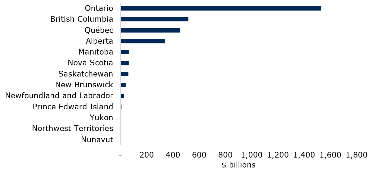
Source: OSFI calculations based on 2026 CRR (DC1).
Text description
| Province / territory | Banking exposure ($B) |
|---|---|
| Nunavut | 0.9 |
| Northwest Territories | 2.3 |
| Yukon | 0.7 |
| Prince Edward Island | 8.6 |
| Newfoundland and Labrador | 28.6 |
| New Brunswick | 39.0 |
| Saskatchewan | 59.6 |
| Nova Scotia | 62.6 |
| Manitoba | 63.6 |
| Alberta | 339.2 |
| Québec | 456.7 |
| British Columbia | 516.9 |
| Ontario | 1,531.1 |
Insurance data show a similar pattern. Insurers reported approximately $12 trillion in TIV, with Ontario accounting for approximately $5.4 trillion. Québec, British Columbia, and Alberta each accounted for approximately $1.7 trillion to $1.8 trillion. Together, these results highlight significant DTI and insurance concentrations in Canada's largest economic and population centres. See Figure 2.2 for insurance TIV by province.
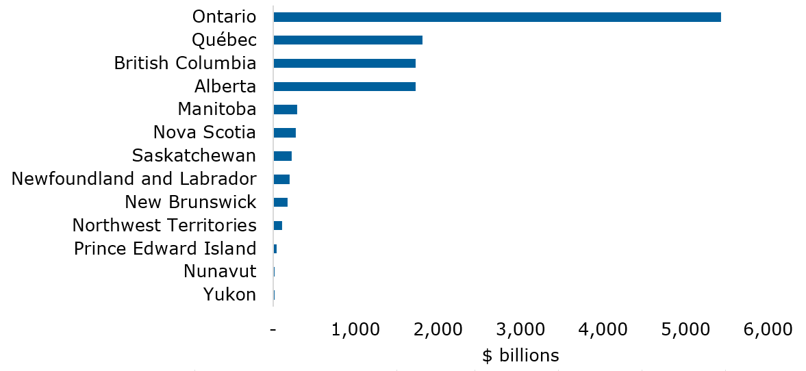
Source: OSFI calculations based on 2026 CRR (IC1).
Text description
| Province / territory | Total insured value ($B) |
|---|---|
| Yukon | 16.36 |
| Nunavut | 21.15 |
| Prince Edward Island | 43.54 |
| Northwest Territories | 112.83 |
| New Brunswick | 179.97 |
| Newfoundland and Labrador | 201.85 |
| Saskatchewan | 227.04 |
| Nova Scotia | 275.05 |
| Manitoba | 293.71 |
| Alberta | 1,729.95 |
| British Columbia | 1,730.17 |
| Québec | 1,811.38 |
| Ontario | 5,425.96 |
Geographic concentration provides an important starting point for analysis. However, location alone does not indicate physical risk. Exposures should be considered alongside the hazards to which they could be subject.
2.2 Hazard overlays reveal different risk profiles
To better understand physical risk concentrations, we overlay DTI exposure data with flood and wildfire hazard information from MSCI, NRCan and ECCC.
This analysis highlights how concentrations vary by hazard, risk area, and geography (see Figure 2.3). About $3 trillion in DTI exposure could be mapped at the forward sortation area (FSA) level to the MSCI, NRCan and ECCC datasets. Approximately 22% of the mapped exposure fell within high- or very high-risk pluvial-flood hazard areas.Footnote 4 By comparison, 12% fell within high- or very high-risk wildfire hazard areas.Footnote 5 The picture changed when we include moderate-risk hazard areas. Wildfire and pluvial-flood exposure represented 62% and 48% of mapped exposure, respectively. These results illustrate how the proportion of exposure identified as being at risk varies depending on the risk categories included in the analysis.Footnote 6
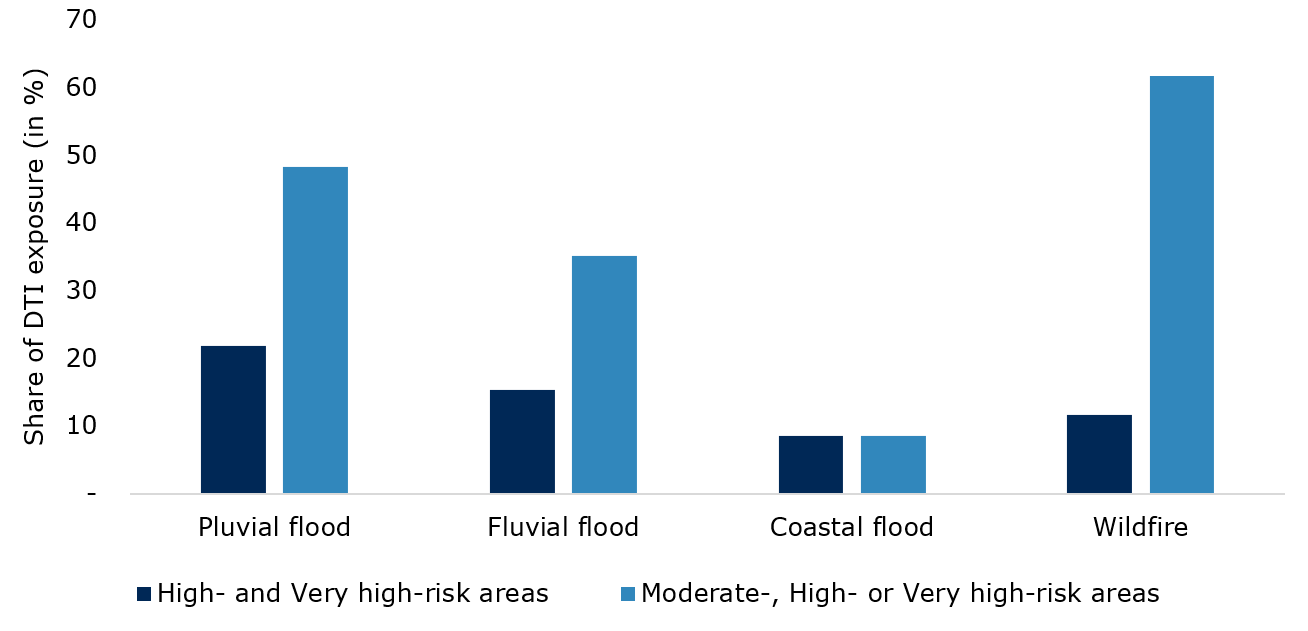
Source: OSFI calculations based on 2026 CRR (DC1), MSCI, NRCan and ECCC datasets. Based on 2050 climate scenarios. Flood risk is based on average annual loss. Wildfire risk is based on the Buildup Index and NRCan Wildland-Urban Interface layer.
Text description
| no data | Pluvial flood | Fluvial flood | Coastal flood | Wildfire |
|---|---|---|---|---|
| High- and Very high-risk areas | 21.80 | 15.30 | 8.60 | 11.70 |
| Moderate-, High- or Very high-risk areas | 48.30 | 35.20 | 8.60 | 61.80 |
Geographic concentrations also varied by hazard (See Figure 2.4):
- British Columbia had the largest overall higher-risk hazard exposure, largely driven by wildfire
- Québec and Ontario had the largest concentrations of pluvial-flood exposure
- Alberta had material exposure to both pluvial and fluvial flood
- Overall, the geographic concentration of exposure differed significantly by hazard and province
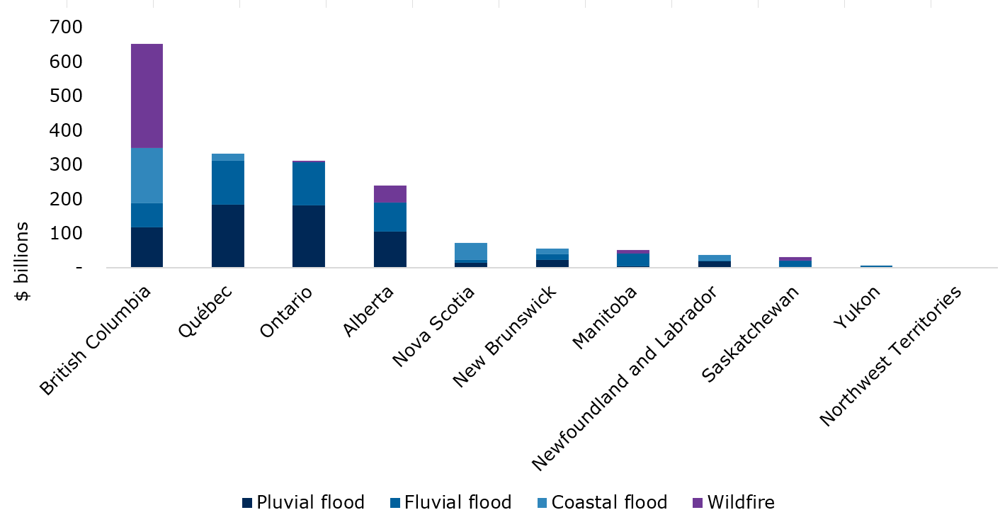
Source: OSFI calculations based on 2026 CRR (DC1), MSCI, NRCan and ECCC datasets. Based on 2050 climate scenarios. Flood risk is based on average annual loss. Wildfire risk is based on the Buildup Index and NRCan Wildland-Urban Interface layer.
Text description
| no data | Pluvial flood | Fluvial flood | Coastal flood | Wildfire |
|---|---|---|---|---|
| British Columbia | 117.91 | 69.69 | 162.12 | 302.70 |
| Québec | 184.74 | 127.80 | 20.59 | no data - |
| Ontario | 182.61 | 125.37 | 1.03 | 3.90 |
| Alberta | 106.83 | 83.90 | no data - | 49.60 |
| Nova Scotia | 14.44 | 8.53 | 49.85 | no data - |
| New Brunswick | 23.95 | 15.71 | 16.63 | no data - |
| Manitoba | 5.29 | 35.71 | 0.39 | 11.40 |
| Newfoundland and Labrador | 19.19 | 2.21 | 15.56 | no data - |
| Saskatchewan | 2.69 | 19.16 | no data - | 10.40 |
| Yukon | 3.19 | 3.19 | no data - | no data - |
| Northwest Territories | no data - | no data - | no data - | 0.70 |
The above results show that physical risk concentrations differ across hazards and regions. Understanding these differences can help identify potential vulnerabilities and guide further analysis.
2.3 Residential real estate connects multiple risk channels
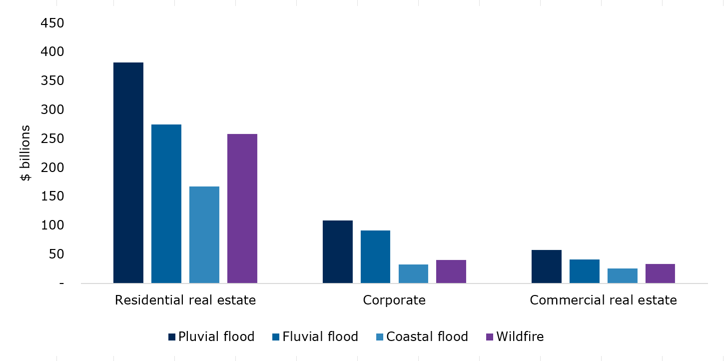
Residential real estate represented the largest DTI exposure in higher-risk hazard areas across all hazards examined. Of total DTI exposure in high- and very high-risk areas, residential real estate accounted for 58% for pluvial flood, 56% for fluvial flood, 63% for coastal flood, and 68% for wildfire. Corporate lending and commercial real estate also represented material exposures, although their relative importance varied across hazards (see Figure 2.5).
Source: OSFI calculations based on 2026 CRR (DC1), MSCI, NRCan and ECCC datasets. Based on 2050 climate scenarios. Flood risk is based on average annual loss. Wildfire risk is based on the Buildup Index and NRCan Wildland-Urban Interface layer.
Text description
| no data | Residential real estate | Corporate | Commercial real estate |
|---|---|---|---|
| Pluvial flood | 382.4 | 108.52 | 57.55 |
| Fluvial flood | 274.56 | 91.2 | 41.39 |
| Coastal flood | 167.19 | 32.42 | 25.94 |
| Wildfire | 258.8 | 40.7 | 33.4 |
The significant exposure of residential real estate helps illustrate physical risk as a financial risk. Damage to residential property can affect households, mortgage collateral, insurance claims, rebuilding costs, and the availability and affordability of insurance. As a result, residential real estate shows how a severe physical event could affect multiple parts of the financial system simultaneously.
Commercial real estate and corporate lending also represent important exposures. However, their potential financial impacts are more heterogeneous because they depend on business operations, property characteristics, supply chains, business-continuity arrangements, and insurance coverage.
2.4 Claims and modeled losses provide complementary perspectives
Insurance data provide additional perspectives on physical risk through claims experience and probable maximum loss (PML) estimates.Footnote 7 Claims data provide evidence of losses that have already occurred, while PML estimates provide a forward-looking view of potential losses from severe events. Together, they complement the analysis of exposure to physical hazards by providing information on their financial consequences.
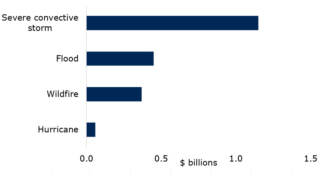
Claims patterns differed across perils. Severe convective storm generated the largest reported claims during the year (see Figure 2.6). Flood generated approximately 16,400 claims, averaging about $27,000 per paid claim, while wildfire generated approximately 2,300 claims, averaging about $159,000 per paid claim, almost six times the average flood claim.
Source: OSFI calculations based on 2026 CRR (IC1).
Text description
| Peril | Claims paid ($B) |
|---|---|
| Hurricane | 0.1 |
| Wildfire | 0.4 |
| Flood | 0.5 |
| Severe convective storm | 1.2 |
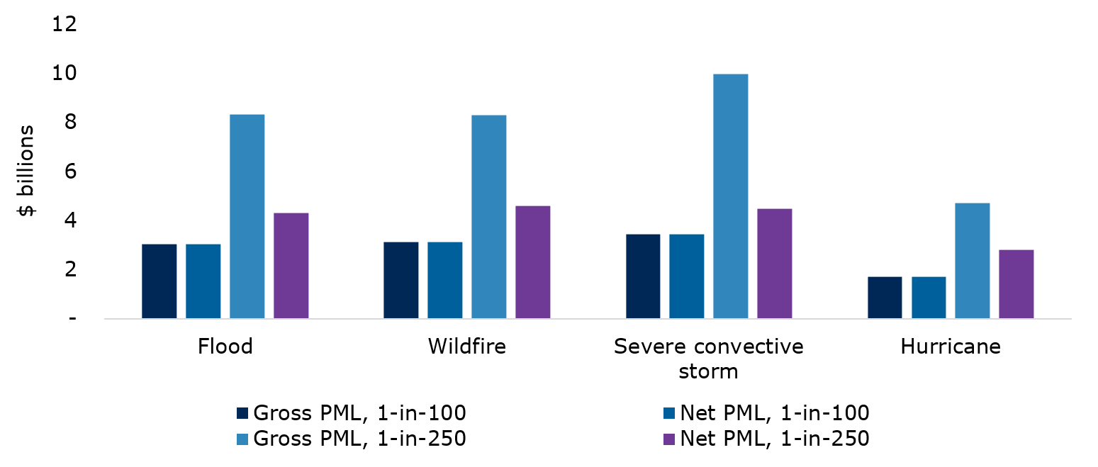
PML estimates complement claims experience by providing a forward-looking view of potential losses from more severe events. Severe convective storm generates the largest gross modeled losses. Wildfire and hurricane losses increase most sharply under more severe scenarios. Differences between PMLs gross and net of reinsurance also illustrate the critical role of reinsurance and other risk-mitigation arrangements (see Figure 2.7).
Source: OSFI calculations based on 2026 CRR (IC1).
Text description
| no data | Flood | Wildfire | Severe convective storm | Hurricane |
|---|---|---|---|---|
| Gross PML, 1-in-100 | 4.96 | 4.19 | 6.27 | 2.45 |
| Net PML, 1-in-100 | 3.03 | 3.13 | 3.43 | 1.72 |
| Gross PML, 1-in-250 | 8.31 | 8.28 | 9.95 | 4.70 |
| Net PML, 1-in-250 | 4.32 | 4.60 | 4.49 | 2.82 |
Together, hazard overlays, claims experience, and modeled losses provide complementary perspectives on physical risk. Different perils emerge as most significant depending on the indicator examined. While no single indicator captures vulnerability or predicts future losses, the usage of various indicators helps identify concentrations and potential vulnerabilities that could warrant further analysis.
2.5 Putting the metrics in context
The metrics in this section provide different perspectives on physical risk. They do not, on their own, establish vulnerability or predict future financial losses.
Location in a higher-risk hazard area does not necessarily result in financial loss. Financial impacts also depend on factors such as the hazard severity, asset characteristics and resilience, insurance coverage, adaptation measures, and risk-management practices.
Similarly, claims data reflect events that occurred during the reporting period, while PML estimates represent modeled losses under specified scenarios. Neither should be interpreted as a forecast of future losses.
Taken together, analysis of exposure to physical hazards, claims experience, and modeled losses provide complementary perspectives on potential vulnerabilities. The analysis highlights where exposures and physical hazards intersect and where further analysis might be warranted. Broader prudential implications are considered in Section 4.
3. Transition risk – exposure to a changing economy
This section examines where transition-vulnerable sectorFootnote 8 (TVS) exposures are concentrated. It also examines financed emissions, emissions intensity, and maturity. Each dimension provides a different perspective on transition-related vulnerabilities. Exposure identifies concentrations. Financed emissions and emissions intensity characterize emissions associated with financing activities. Maturity provides a time-horizon perspective. Considered together, these perspectives provide a more complete view of potential transition-related vulnerabilities.
3.1 TVS exposures are concentrated
DTIs reported approximately $448 billion of TVS exposure, representing 11% of the relevant $4.2 trillion portfolio. Insurers reported about $120 billion, representing approximately 30% of their relevant portfolio. Thus, DTIs reported larger exposures in absolute terms, while TVS represented a larger share of insurers' portfolios.
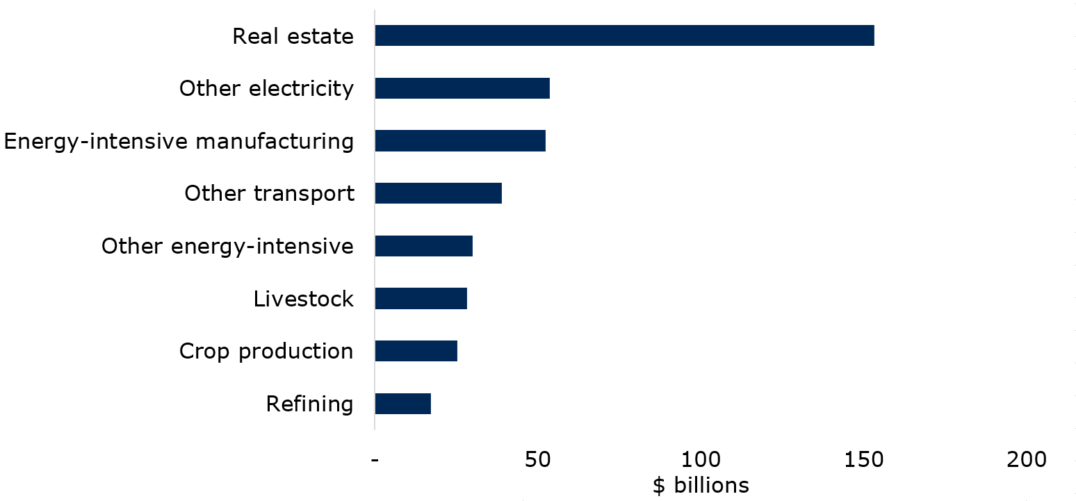
A relatively small number of sectors accounted for most TVS exposure. For DTIs, the five largest sectors represented more than 70% of TVS exposure, led by real estate, other electricityFootnote 9, and energy-intensive manufacturing (see Figure 3.1). For insurers, other electricity, real estate, and refining together accounted for about 50% of TVS exposures, with other electricity representing the largest exposure at approximately $31 billion (see Figure 3.2).
Source: OSFI calculations based on 2026 CRR (DC2).
Text description
| no data | Exposure |
|---|---|
| Oil sands | 0.12 |
| Coal | 0.19 |
| Rail transport | 3.39 |
| Fossil-fuel electricity | 4.79 |
| Air transport | 6.67 |
| Oil support | 8.01 |
| Oil extraction | 11.98 |
| Natural gas | 14.00 |
| Refining | 17.11 |
| Crop production | 25.19 |
| Livestock | 28.24 |
| Other energy-intensive | 29.96 |
| Other transport | 38.90 |
| Energy-intensive manufacturing | 52.47 |
| Other electricity | 53.71 |
| Real estate | 153.14 |
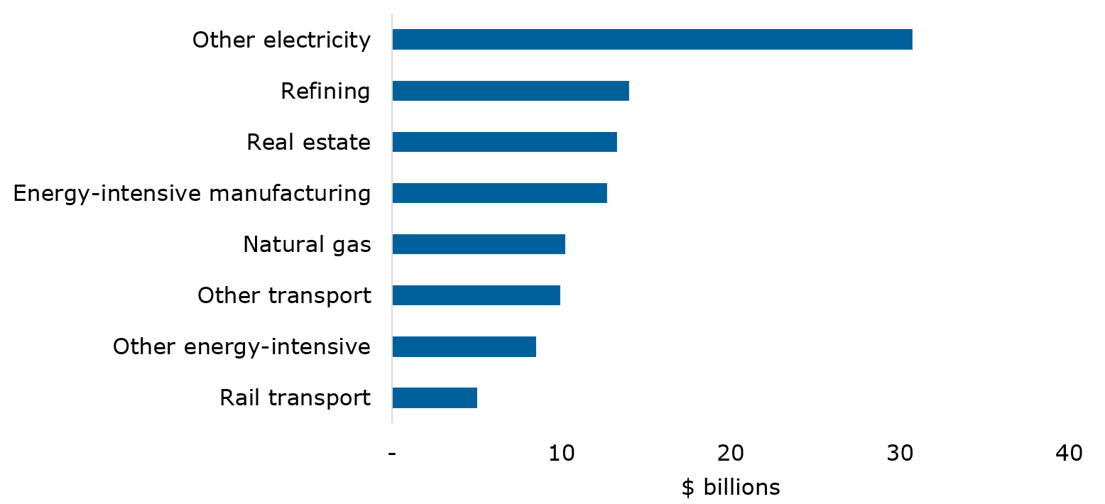
Source: OSFI calculations based on 2026 CRR (IC2).
Text description
| no data | Exposure |
|---|---|
| Livestock | 0.11 |
| Coal | 0.38 |
| Crop production | 0.42 |
| Oil sands | 0.63 |
| Fossil-fuel electricity | 2.05 |
| Oil support | 2.06 |
| Oil extraction | 3.81 |
| Air transport | 4.81 |
| Rail transport | 5.01 |
| Other energy-intensive | 8.50 |
| Other transport | 9.93 |
| Natural gas | 10.24 |
| Energy-intensive manufacturing | 12.70 |
| Real estate | 13.29 |
| Refining | 13.99 |
| Other electricity | 30.74 |
Asset-class composition also differed. Corporate loans accounted for most DTI exposure (82%), while publicly traded corporate bonds and debentures accounted for most insurer exposure (87%). These differences could affect how transition-related risks emerge, how long they remain on balance sheets, and how quickly institutions can respond to changing conditions.
3.2 Exposure and emissions reveal different risk profiles
Financed emissions provide a different perspective on exposure. Exposure identifies where concentrations exist, while financed emissions and emissions intensity provide information on the emissions associated with those exposures. Together, these metrics provide a more complete picture of transition-related risks.
DTIs reported about 110 million tonnes of carbon dioxide equivalent (MtCO₂e) of Scope 1 and 2 financed emissionsFootnote 10 across the TVS examined. Life and P&C insurers reported about 16 MtCO₂e.Footnote 11 DTIs therefore reported a substantially larger financed-emissions footprint. DTIs also reported approximately double the financed-emissions intensity of insurers. Across the TVS analyzed, financed-emissions intensity averaged about 245 tCO₂e per $1 million of exposure for DTIs and about 145 tCO₂e for insurers.
Sector-level results show why exposure and emissions intensity should be considered together. For DTIs, real estate represented the largest exposure at about $154 billion, or 34% of TVS exposure. However, its emissions intensity remained well below the DTI average. In contrast, smaller sectors such as livestock, oil extraction, and fossil-fuel electricity reported much higher emissions intensity despite lower exposures (see Figure 3.3).
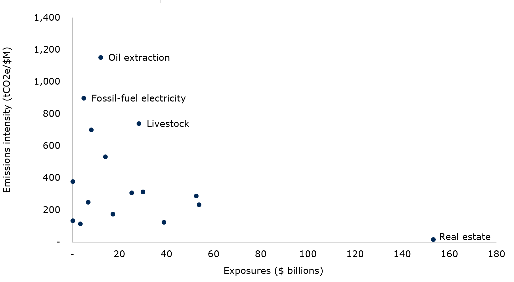
Source: OSFI calculations based on 2026 CRR (DC2).
Text description
| no data | Exposure | Intensity |
|---|---|---|
| Real estate | 153.14 | 17.15 |
| Other electricity | 53.71 | 234.49 |
| Energy-intensive manufacturing | 52.47 | 288.03 |
| Other transport | 38.90 | 123.61 |
| Other energy-intensive | 29.96 | 313.11 |
| Livestock | 28.24 | 739.91 |
| Crop production | 25.19 | 308.69 |
| Refining | 17.11 | 174.71 |
| Natural gas | 14.00 | 532.79 |
| Oil extraction | 11.98 | 1,151.90 |
| Oil support | 8.01 | 700.80 |
| Air transport | 6.67 | 249.58 |
| Fossil-fuel electricity | 4.79 | 898.71 |
| Rail transport | 3.39 | 114.01 |
| Coal | 0.19 | 133.18 |
| Oil sands | 0.12 | 378.17 |
| Other | 893.99 | 38.11 |
Insurers showed a similar distinction between exposure and intensity. Other electricity represented the largest insurer exposure at about $31 billion, while fossil-fuel electricity and coal reported the highest emissions intensity. These results show that the largest exposures are not always the most emission intensive. Exposure and emissions intensity therefore provide different perspectives on transition-related vulnerabilities.
3.3 Maturity and data quality provide complementary perspectives
Maturity provides a time-horizon perspective on transition-related risk. Approximately 0.5% of DTI exposure to TVS had a remaining maturity of ten years or more, compared with slightly over 40% for insurers. These differences largely reflect insurers' holdings of longer-dated corporate bonds and debentures.
Longer maturities do not indicate greater risk on their own. However, they could extend the period during which institutions remain exposed to transition-related developments.
Financed-emissions estimates continue to rely on varying degrees of reported data, estimates, and proxies. As a result, underlying data quality remains an important consideration when interpreting results. Differences in data quality can affect comparisons across institutions, asset classes, and reporting periods.
Neither maturity nor data quality assess transition risk directly. However, both provide important context when interpreting exposure, emissions, and intensity results.
3.4 Putting the metrics in context
The metrics in this section identify concentrations, emissions characteristics, and maturity profiles. However, they do not individually establish vulnerability or estimate future losses. Exposure to a TVS does not mean every business within this sector faces the same risks. Similarly, higher financed emissions or emissions intensity are not, on their own, indicative of a counterparty's transition strategy, preparedness, financial strength, or ability to adapt.
Metrics are most informative when considered together. While not one tells the whole story, they help reveal different dimensions of transition-related risk and support prudential analysis. We discuss broader prudential implications in Section 4.
4. Prudential insights and next steps
The CRR contains data about exposures, concentrations, insurance claims, and modeled losses - the CRR does not contain estimates of expected future losses. The CRR helps us understand where climate-related risk drivers intersect with financial exposures and where further analysis might be warranted.
4.1 Key prudential insights
a. Concentration matters
The results show material concentrations across regions, hazards, asset classes, and sectors. Physical risk exposures remain concentrated in specific geographies and portfolios, while TVS exposures remain concentrated in a relatively small number of sectors.
Our analysis also highlights important differences between DTIs and insurers. DTIs reported larger transition-related exposures and financed emissions in absolute terms, while TVS represented a larger share of insurers' portfolios and included materially longer maturities. These findings highlight the importance of considering the location, composition, and duration of exposures rather than aggregate amounts alone.
b. Multiple metrics provide different perspectives on risk
The report combines multiple measures to examine climate-related financial risks. Hazard overlays, claims experience, and PML estimates provide different perspectives on potential vulnerability from physical risks. Exposure, financed emissions, emissions intensity, maturity, and underlying data quality each highlight different dimensions of transition risk.
While no single metric, insight or consideration tells the whole story, together they provide complementary perspectives on potential prudential vulnerabilities. They are more informative when interpreted together.
c. Common exposures can create system-wide connections
Certain exposures can affect multiple parts of the financial system simultaneously. Residential real estate provides the clearest example. A severe physical event could affect households through property damage, DTIs through borrower repayment capacity and collateral values, and insurers through claims and losses.
Some portfolios are also exposed to both physical and transition-related risk drivers. Identifying these common exposures can help focus analysis on areas where multiple transmission channels could intersect.
d. Insurance conditions are an important part of the bank–insurer nexus
Insurance can mitigate the financial effects of physical events. However, changes in insurance availability, affordability, or coverage could also affect households, property values, collateral, and credit exposures.
Understanding this nexus requires sufficiently granular and comparable information across DTIs and insurers. Greater alignment in geographic data would support analysis of where banking exposures, insured assets, and physical hazards are concentrated in the same locations.
4.2 Next steps
The next phase of CRR development will focus on improving data quality, deepening analysis, and strengthening the use of CRR information in prudential supervision.
a. Improve the data
We will continue to improve the completeness, consistency, and usefulness of CRR information, including geographic information, sector classification, financed-emissions reporting, and underlying data quality measures.
Starting with the 2027–2028 reporting cycle, we intend to seek FSA-level geographic information from property and casualty insurers. This enhancement would improve alignment with DTI data and support analysis of where lending, collateral, insured exposures, and insurance losses intersect.
We also intend to implement the Partnership for Carbon Accounting Financials 2025 Standard for financed-emissions reporting, supported by implementation guidance. We will document methodological changes so users can distinguish changes in exposure and emissions from changes from the revised standard.
b. Deepen the analysis
As the CRR dataset grows, we will continue to strengthen the analysis of:
- geographic, asset-class, and sectoral concentrations
- intersections between financial exposures and external hazard information
- linkages between DTI and insurers
- portfolios exposed to physical and transition risk drivers
- changes over time
A longer and more consistent time series will improve our ability to identify emerging concentrations and vulnerabilities.
c. Support prudential supervision
We will continue to use CRR information alongside other supervisory data and analyses. The CRR helps identify where material exposures, concentrations, and transmission channels warrant closer examination.
The foundation is now in place. As the dataset expands and analysis matures, the CRR will continue to turn climate-risk data into prudential insight.
Appendix A: Lessons learned from the second reporting cycle
The second CRR reporting cycle provides insight into institutions' ability to collect, manage, and report climate-related information. Three broad observations emerged from the 2026 reporting cycle.
a. Reporting processes continue to mature
Institutions reporting for a second cycle generally demonstrated greater familiarity with CRR requirements and experienced fewer filing issues. Most operational challenges occurred among first-time filers and primarily involved submission processes, formatting requirements, and technical reporting specifications.
b. Data quality remains an important challenge
Some climate-related metrics continue to rely on estimates and proxies where institution- or counterparty-specific information is unavailable. Financed-emissions reporting using Partnership for Carbon Accounting Financials scores illustrates this challenge. Differences in underlying data quality can affect comparability across institutions, asset classes, and reporting periods. Results should therefore be interpreted alongside data quality indicators and reporting coverage.
c. Granular data enable more sophisticated analysis
Granular geographic information allows reported exposures to be linked with external hazard datasets and supports a more detailed analysis of physical and catastrophic risk concentrations. The 2026 reporting cycle enabled the use of external hazard overlays to examine where financial exposures intersect with flood and wildfire hazards. Continued improvements in geographic information should support increasingly detailed analysis over time.
Looking ahead, the reporting process and the underlying climate-risk information will continue to mature at different rates. Future enhancements will focus on improving data quality, increasing geographic granularity, and supporting more sophisticated analysis of climate-related concentrations and vulnerabilities across the financial system.